
Empirical Approach for Modelling Tree Phenology in Mixed Forests Using Remote Sensing


1
Department of Forest Ecology and Management, Swedish University of Agricultural Sciences, Skogsmarksgränd 17, 901 83 Umeå, Sweden
2
Department of Forest Ecology, Slovenian Forestry Institute, Večna Pot 2, 1000 Ljubljana, Slovenia
3
Meteorology and Hydrology Office, Slovenian Environment Agency, Vojkova 1b, 1000 Ljubljana, Slovenia
*
Author to whom correspondence should be addressed.
Remote Sens. 2021, 13(15), 3015; https://doi.org/10.3390/rs13153015
Submission received: 23 June 2021
/
Revised: 26 July 2021
/
Accepted: 29 July 2021
/
Published: 1 August 2021
(This article belongs to the Special Issue Vegetation Phenology from Remote Sensing data: Monitoring, Mapping, and Modelling)
Abstract
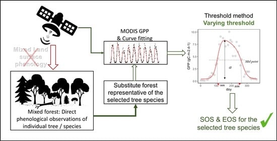
:Phenological events are good indicators of the effects of climate change, since phenological phases are sensitive to changes in environmental conditions. Although several national phenological networks monitor the phenology of different plant species, direct observations can only be conducted on individual trees, which cannot be easily extended over large and continuous areas. Remote sensing has often been applied to model phenology for large areas, focusing mostly on pure forests in which it is relatively easier to match vegetation indices with ground observations. In mixed forests, phenology modelling from remote sensing is often limited to land surface phenology, which consists of an overall phenology of all tree species present in a pixel. The potential of remote sensing for modelling the phenology of individual tree species in mixed forests remains underexplored. In this study, we applied the seasonal midpoint (SM) method with MODIS GPP to model the start of season (SOS) and the end of season (EOS) of six different tree species in Slovenian mixed forests. First, substitute locations were identified for each combination of observation station and plant species based on similar environmental conditions (aspect, slope, and altitude) and tree species of interest, and used to retrieve the remote sensing information used in the SM method after fitting the best of a Gaussian and two double logistic functions to each year of GPP time series. Then, the best thresholds were identified for SOS and EOS, and the results were validated using cross-validation. The results show clearly that the usual threshold of 0.5 is not best in most cases, especially for estimating the EOS. Despite the difficulty in modelling the phenology of different tree species in a mixed forest using remote sensing, it was possible to estimate SOS and EOS with moderate errors as low as <8 days (Fagus sylvatica and Tilia sp.) and <10 days (Fagus sylvatica and Populus tremula), respectively.
1. Introduction
Reliable phenological observations, achieved through either direct visual human observations in phenology networks, near-surface measurements using phenology cameras and unmanned aerial vehicles, or remote sensing via satellites [1], are important for anticipating the effects of climate change on tree phenology in forests. In fact, tree phenological phases mirror environmental conditions and thus can respond to variations in climate, making them good indicators of the effects of climate change when long series of phenological observations exist, as they can reveal some trends in the timing of spring and autumn phenological events [2,3].
Long-term phenological observations in trees, including spring events such as leaf unfolding and autumnal events of leaf colouring, have shown that a rise in global temperature generally leads to earlier timing of spring events [4,5,6]. Leaf phenology is a major determinant of water and CO2 fluxes, and several studies clearly showed that growing season length controls net ecosystem primary productivity and that phenological shifts already modified the annual carbon cycle of terrestrial ecosystems [7,8].
Although many national phenological monitoring networks have their phenological stations equally distributed over altitude, slope, and aspect, most of the stations are either outside the forest or on the forest edge due to accessibility and other practical reasons [4,9]. This could have implications for the observed tree phenology and the generalisations resulting from these observations at national or regional scales [10].
Direct observations on the ground can provide phenological characteristics of the different plant species present at a given location. However, they are unable to provide continuous phenology characteristics for a given geographic area [11]. On the other hand, satellite data can help estimate and monitor phenological characteristics over extended areas, even though these estimations are always more generalised than direct observations of individual plant phenology [12,13].
Phenology modelling using remote sensing typically makes use of vegetation indices such as the normalised difference vegetation index (NDVI), the enhanced vegetation index (EVI) and leaf area index (LAI) [1,14]. The choice of remote sensing data source requires a compromise between their spatial resolution, their temporal resolution, and their time span. Landsat missions provide long records of data with 30 m spatial resolution, but their temporal resolution is around 16 days, making it more challenging to reconstruct continuous data, especially when large data gaps are present. For this reason, several phenology modelling studies turned to moderate and low resolution satellites (>250 m) provided by the advanced very-high-resolution radiometer (AVHRR) and the moderate-resolution imaging spectroradiometer (MODIS) [15,16,17]. Some studies demonstrated the adequacy of gross primary production (GPP) for modelling plant phenology [18,19], making the MODIS GPP product a useful and yet underexplored data source to that end, considering their high temporal resolution of 8 days.
To derive phenological characteristics from remote sensing data, seasonality in the satellite data time series is essential. Different factors affect the seasonality observed in the remote sensing data. These factors include noise and extended gaps in the data [20,21], but also low temporal resolution [22]. It is therefore usual practice to apply mathematical functions to smooth or fit a curve to the time series of remote sensing data and provide continuous data useful for modelling the phenology. These methods include logistic and improved logistic models [23,24,25,26], Gaussian functions [27], quadratic functions and non-linear spherical models [28,29], Savitzky–Golay filters [30], polynomial functions [31], discrete Fourier series [11] and machine learning-based algorithms [32]. After reconstructing continuous data, phenological characteristics are often extracted following different approaches [13], mainly threshold-based methods [11,33], the moving averages approach [34], the inflection point method [23] and the time of maximum increase [33,35]. The data reconstruction algorithm and phenology extraction methods chosen would greatly affect the modelled phenology. The simplicity and flexibility of threshold-based methods make them particularly popular. In addition, they were found to predict the start of season (SOS) more accurately than other methods in different forests in Europe [11], North America [36] and China [37].
Phenology modelling studies using remote sensing mostly focused on pure deciduous tree species and showed a good correlation with ground observations. In areas with mixed plant species, the phenology of individual plant species are all grouped under a unique “pixel ecosystem” phenology, or land surface phenology, which is often investigated instead of the phenology of the individual tree species in most studies dealing with mixed forests [38,39,40]. Land surface phenology is generally found to be more difficult to model in mixed forests compared to pure forests, especially for the end of season (EOS) [41]. The ground observations often used to match remote sensing data for EOS are either the date of leaf colouring or the date of leaf fall depending on plant species [42], which are further difficult to apprehend in mixed forests. To our knowledge, very few (if any) studies modelled the phenology of individual tree species in mixed forests using remote sensing. In fact, with multiple plant species coexisting in the extent of a remote sensing pixel, it is not straightforward to match ground observations with remote sensing information in order to model the phenology of different tree species in a mixed forest.
In this study, we suggest an empirical approach to model the phenology of different tree species in mixed forests. We take advantage of multi-year observations at multiple phenology stations and satellite data to identify the best thresholds for characterizing the phenology (SOS and EOS) for individual tree species at different stations in mixed tree species forests.
2. Materials and Methods
2.1. Study Area and Data Acquisition
2.1.1. Phenological Observations
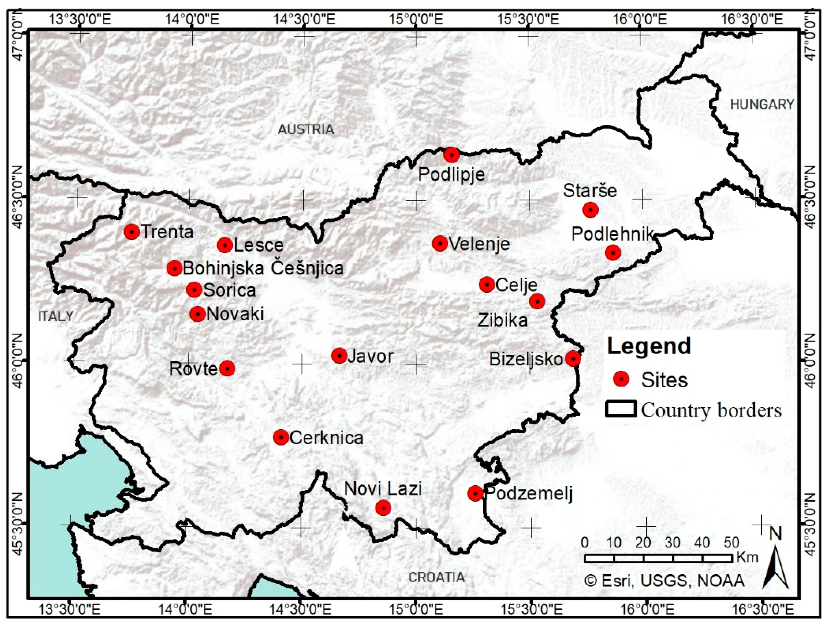
We used data on direct phenological observations of the timing of first leaf unfolding (hereafter termed as start of season, SOS) and general leaf colouring (hereafter termed as end of season, EOS) of selected tree species of the National Phenological Network (NPN) of the Slovenian Environment Agency. Slovenia is characterised by fairly large gradients of climatic factors due to its position between the Alps, the Mediterranean and continental Europe [43,44]. Consequently, a great variety of forest habitats, from the lowlands to the high mountains, can be found in the country [45]. Six broadleaved tree species/groups with more than ten years of available phenological observations provided by the NPN were included in this study: European beech (Fagus sylvatica), silver birch (Betula pendula), lime tree (mainly Tilia platyphyllos), common ash (Fraxinus excelsior), oak (pedunculate oak and sessile oak, i.e., Quercus robur and Quercus petraea, respectively) and aspen (Populus tremula). The phenological data were collected at 17 NPN phenological stations which are distributed throughout Slovenia (Figure 1).
Tree selection and observations were made in accordance with national guidelines [46], which in general follow the World Meteorological Organization (WMO) guidelines for phenological observations [9]. The monitoring of the different phenological events was performed on single individual mature trees for each tree species in natural populations, but more tree species at the same phenological station could be included. The observed trees could be selected in forests (seldom pure), at the forest edge, and in the open area. In spring, the observed period of leaf unfolding and leaf development was approximately four weeks, and during this time, the observations were performed daily. The SOS was recorded when the first regular surfaces of leaves became visible in three to four places on the observed tree. The phase corresponds to Biologische Bundesanstalt, Bundessortenamt und Chemische Industrie code 11 (BBCH11) [47]. The EOS was recorded when at least 50% of the leaves turned yellow on the observed tree (BBCH code 94). Each observed tree was precisely geolocated (longitude, latitude) using a GPS, and station characteristics were noted (elevation, slope, and aspect). The altitude of observed trees ranged from 53 to 820 m above sea level. The period of observation was from 2004 to 2019 for Fagus sylvatica and Quercus sp. at some stations, and from 2010 to 2019 for the other combinations of stations and species.
2.1.2. Remote Sensing Data
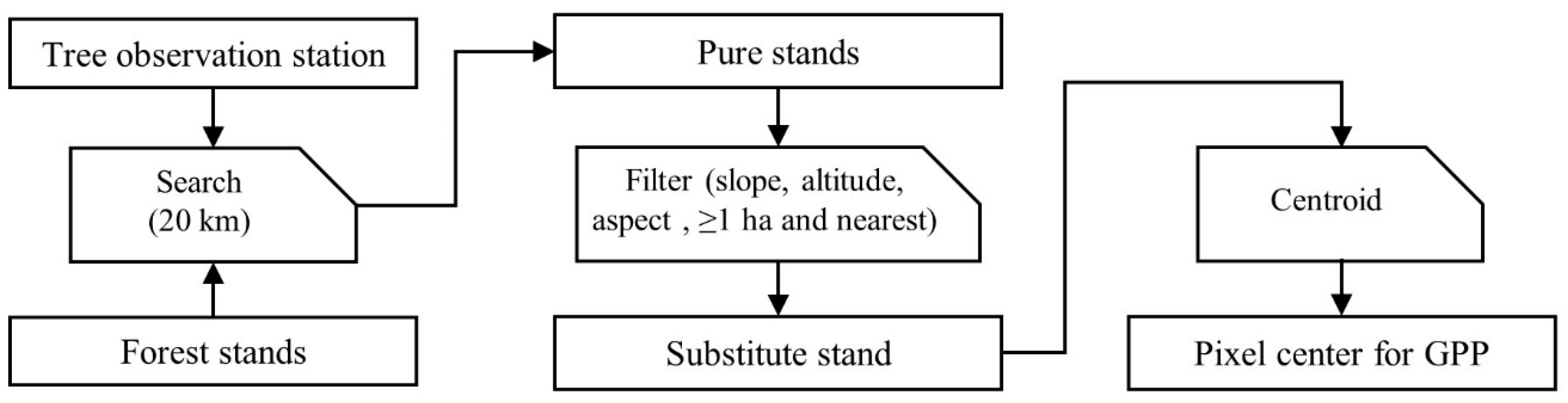
The phenological observations were not always made in the middle of a forest with a significant cover of the plant species being observed. Therefore, to be able to retrieve remote sensing information that reflects ground observations to some extent, the nearest forest stand [48] within a radius of 20 km [49] from the observed tree and with comparable station characteristics was identified. Given the original observation station characteristics (altitude, slope, and aspect), the substitute location used as the centre for the remote sensing data pixel had characteristics not exceeding altitude ± 200 m, slope ± 10°, and aspect ± 1 class (note that aspects represent the standard 1 to 8 categorisation, i.e., N, NE, E, SE, S, SW, W, and NW, with −1 for flat areas). In addition, only stands larger than 1 ha (10,000 m²) qualified for use as a substitute site. This threshold was based on the assumption that if a tree species is represented as nearly pure in 1 ha, it is likely to be present as a secondary species in the rest of the pixel, therefore contributing substantially to the pixel value (note that most of the species included in this study do not form pure stands over extended areas in Slovenia). From the qualifying forest stands satisfying the aforementioned criteria, the nearest stand to the observation station was used as a substitute stand. The centroid of the substitute stand was used to retrieve remote sensing information from Google Earth Engine for the period 2003 to 2020. The previous routine (the generation of the pixel centre from the observation station) applied for each combination of station and tree species using the ArcGIS desktop software (version 10.7.1) is summarised in Figure 2.
We opted for MODIS GPP (8-day aggregate) despite its very coarse spatial resolution (500 m) because the seasonality of GPP was more marked in the mixed forests of this study compared to that of vegetation indices, hence leading to better estimates of phenological events, i.e., SOS and EOS. In addition, the proportion of good quality data available for MODIS GPP (non-missing data after filtering out bad quality pixels) was considerably higher than that of vegetation indices, both from MODIS and Landsat 7, making the seasonality easier to retrieve. However, MODIS (250 m spatial resolution, 8-day temporal resolution) and Landsat 7 ETM+ (30 m spatial resolution, 16-day temporal resolution) derived EVI and NDVI, as well as MODIS LAI (500 m resolution, 4-day temporal resolution) were also tested and reported in this study.
2.2. Data Analysis and Modelling
The 8-day aggregate GPP data were used to reconstruct continuous daily GPP values. First, a fraction of 1/8 was applied to obtain the 8-day average from the downloaded 8-day sums. Then, each year of data was fitted with the best (low RMSE) of (i) a Gaussian function, (ii) a double logistic function after [25], and (iii) another double logistic function after [26]. (ii) and (iii) were performed using the greenbrown package (version 2.5.0) in R (see function equation details in the respective studies), while (i) was performed using non-linear least squares regression also in R, by fitting the following standard Gaussian function:
where k is the peak GPP for the year, t is the day of the year, µ is the day of the year corresponding to the peak of GPP, and σ is the standard deviation.
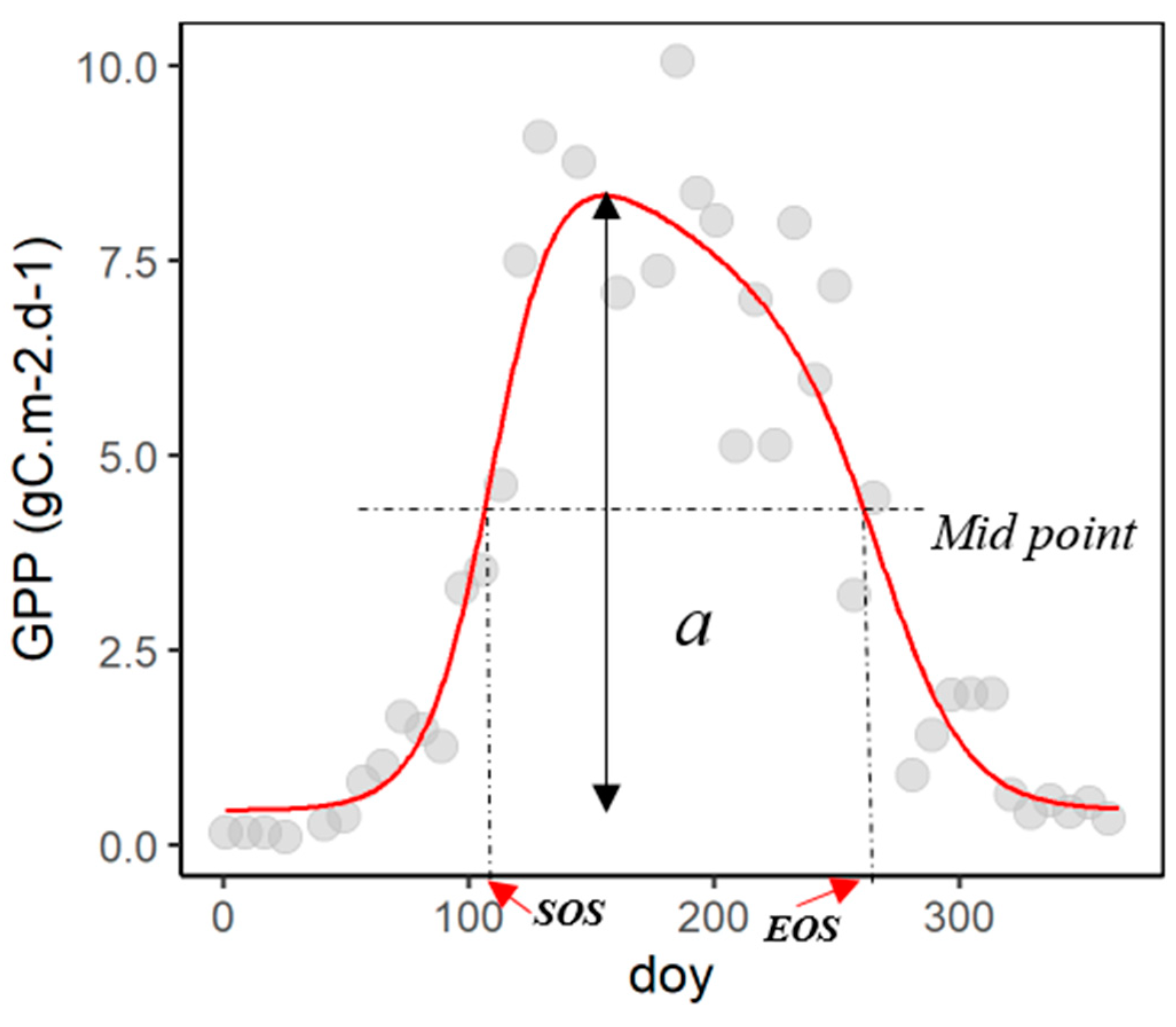
The method used to extract SOS and EOS from the generated daily data is based on the widely used seasonal midpoint (SM) method (illustration in Figure 3). The traditional SM method derives SOS and EOS as the day of the year corresponding to the midpoint (0.5 * amplitude), i.e., SOS on the ascending part of the curve, and EOS on the descending part. For more stable estimates, several studies used a multi-year median of midpoints, instead of a different midpoint for each year [12,37].
In this study, we also used the long-term median threshold. In addition, instead of the traditional midpoint threshold (0.5), we allowed the threshold to vary from 0.05 to 0.95, and to be different for SOS and EOS. This was based on the assumption that in a mixed forest, the species of interest may start contributing significantly to the increase or decrease in GPP at different thresholds compared to a pure forest, depending on the coverage of the species of interest and also the other species present on the site. The best threshold is the one that gives the lowest RMSE of the observed versus modelled SOS or EOS. To test the predictive abilities of the approach, a leave-one-out cross-validation was performed, i.e., estimating each time the best threshold based on all years but one, and then using the holdout year as test data. In that way, all years are used exactly once as validation data when they are not used to train the model. All predictions of holdout year are then put together to calculate RMSE and graphically represent the performance of the model, hence giving a good idea of how well the approach can work in future years.
After the cross-validation, all years were used to determine the best threshold to be applied for future years, for each combination of stations and species. To test the effect of land cover on the best thresholds obtained, fractional land share (% of the pixel) of the species of interest, other broadleaved species, coniferous species, and other land use (including agriculture, grassland, bare land, buildings, etc.) was computed. The best thresholds of 0.45, 0.5 and 0.55 (i.e., ~the traditional threshold) were compared to other best thresholds (<0.45 or >0.55), using the Mann–Whitney test [50,51].
3. Results
3.1. Best Thresholds for the Different Combinations of Stations and Species
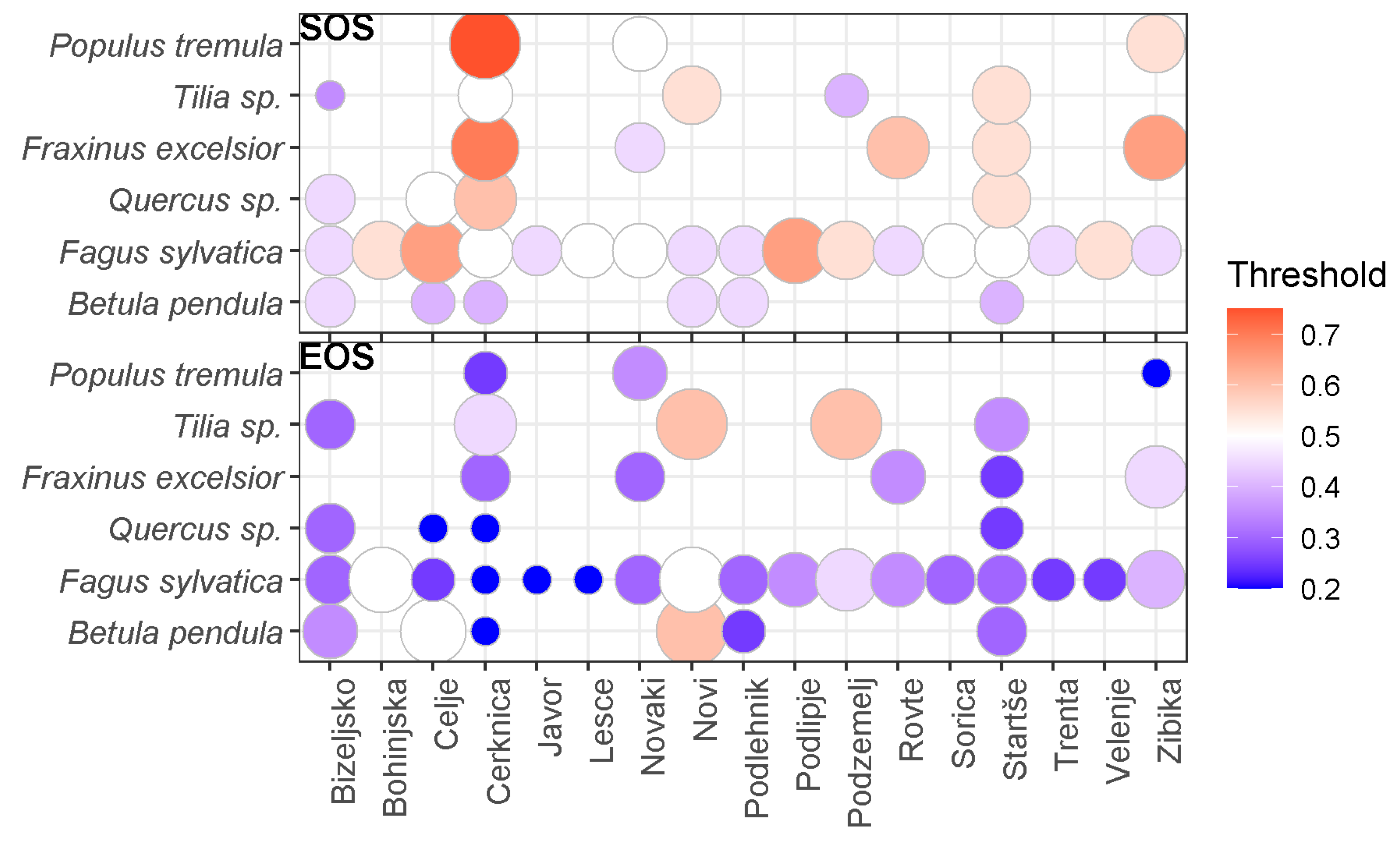
The best thresholds varied substantially between the different combinations of stations and species, and also between SOS and EOS (Figure 4). In general, the best thresholds obtained for SOS are around 0.5, with few combinations of station and species being higher, up to 0.7. For EOS, the best threshold is lower than 0.5 for most combinations of station and species, the minimum being 0.2 for Populus tremula at Zibika, Fagus sylvatica at Cerknica, Javor, Lesce, Betula pendula at Cerknica, and Quercus sp. at Celje and Cerknica. The few exceptions (EOS threshold of 0.5 and 0.6) are Betula pendula at Novi and Celje, Fagus sylvatica at Novi and Bohinjska, and Tilia sp. at Novi and Podzemelj. No plant species stands out consistently as having high or low thresholds of SOS and EOS across all stations.
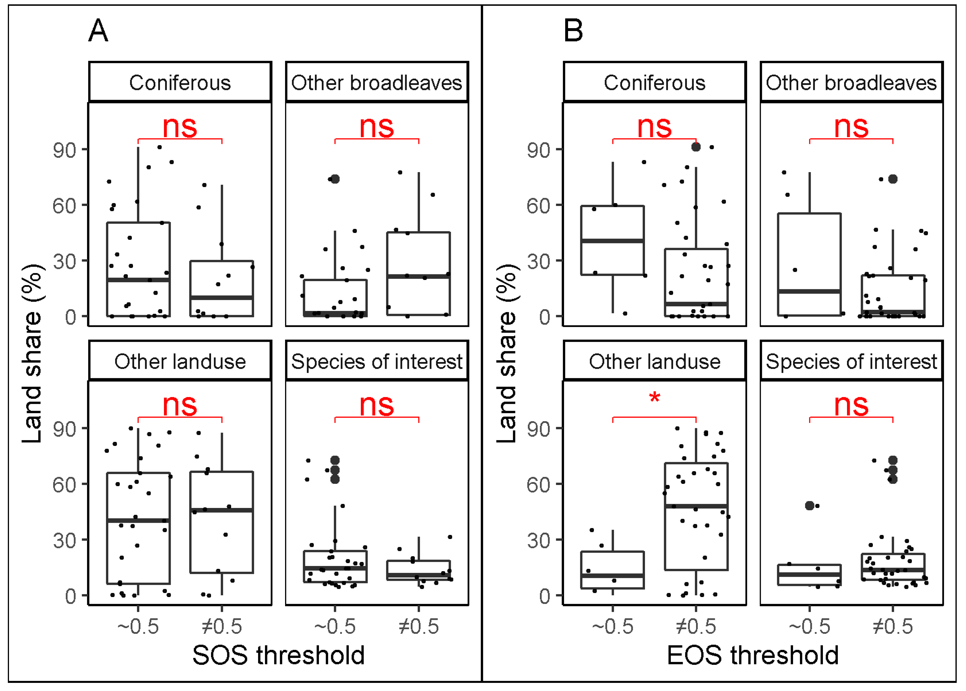
The Mann–Whitney tests comparing the share of different land uses between two groups of best thresholds (close to 0.5 or different from 0.5) are presented in Figure 5. The results suggest that for SOS, the land share of the species of interest, coniferous species, other broadleaved species, and other land use considered separately does not determine if the best threshold would be different from 0.5. For EOS, however, there is a significant difference of land share of other land uses (agriculture, grassland, bare land, buildings, etc.) for the two groups of best thresholds. It appears that combinations of stations and species with higher land shares of other land uses are more likely to result in the best thresholds different from 0.5 (i.e., ≤0.45 and ≥0.55).
3.2. SOS and EOS Estimates from GPP
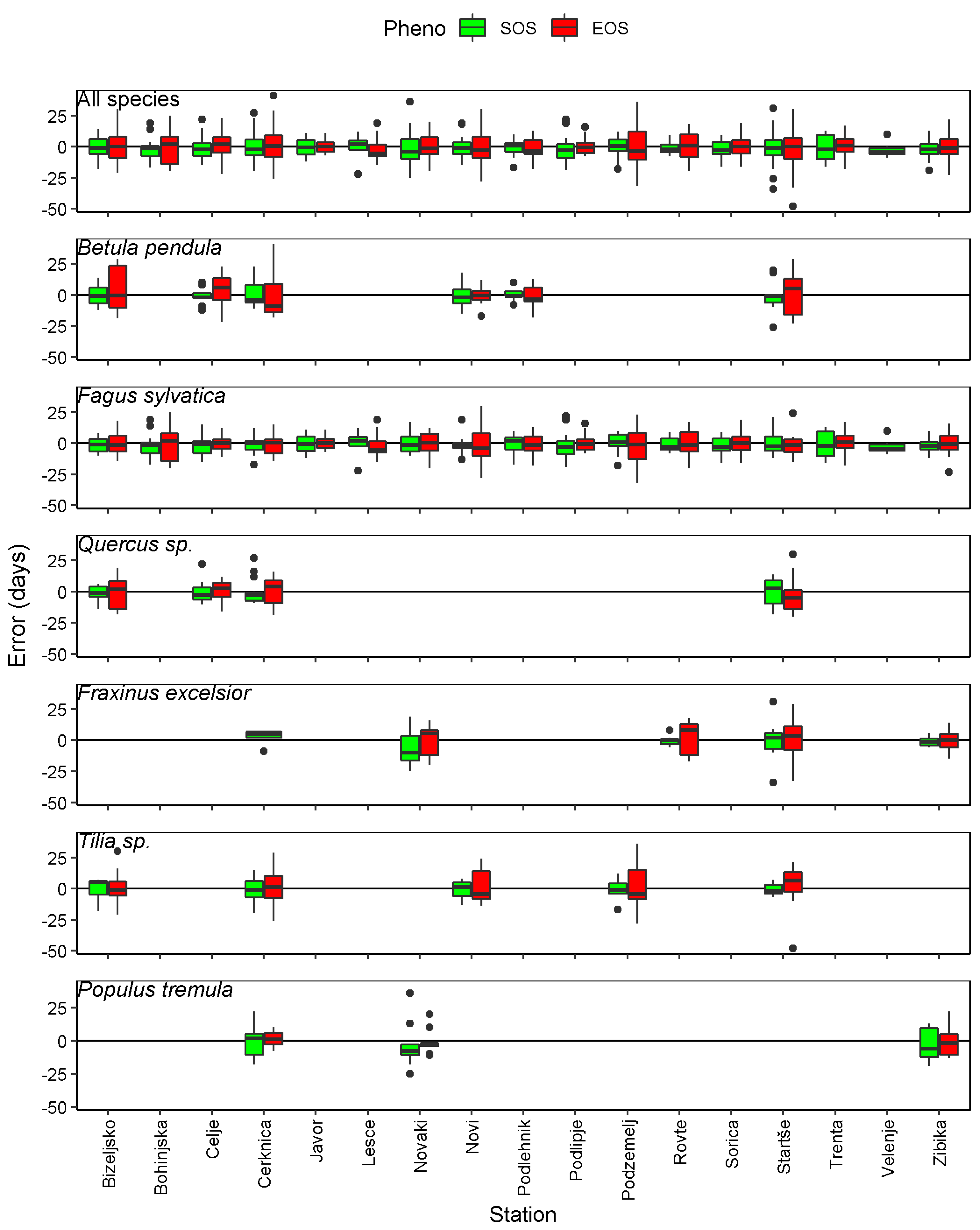
The absolute errors in the modelled SOS and EOS are relatively well spread around the zero-line for all tree species (Figure 6). Errors located above the zero-line represent overestimated SOS or EOS, and errors located below the zero-line represent underestimated SOS or EOS. Overall, the absolute errors are larger for EOS compared to SOS, as denoted by the generally longer boxes. The larger absolute errors of EOS are particularly noticeable at some stations and for specific years, with the highest error at Starše in 2012 for Tilia sp. (error of −48 days).
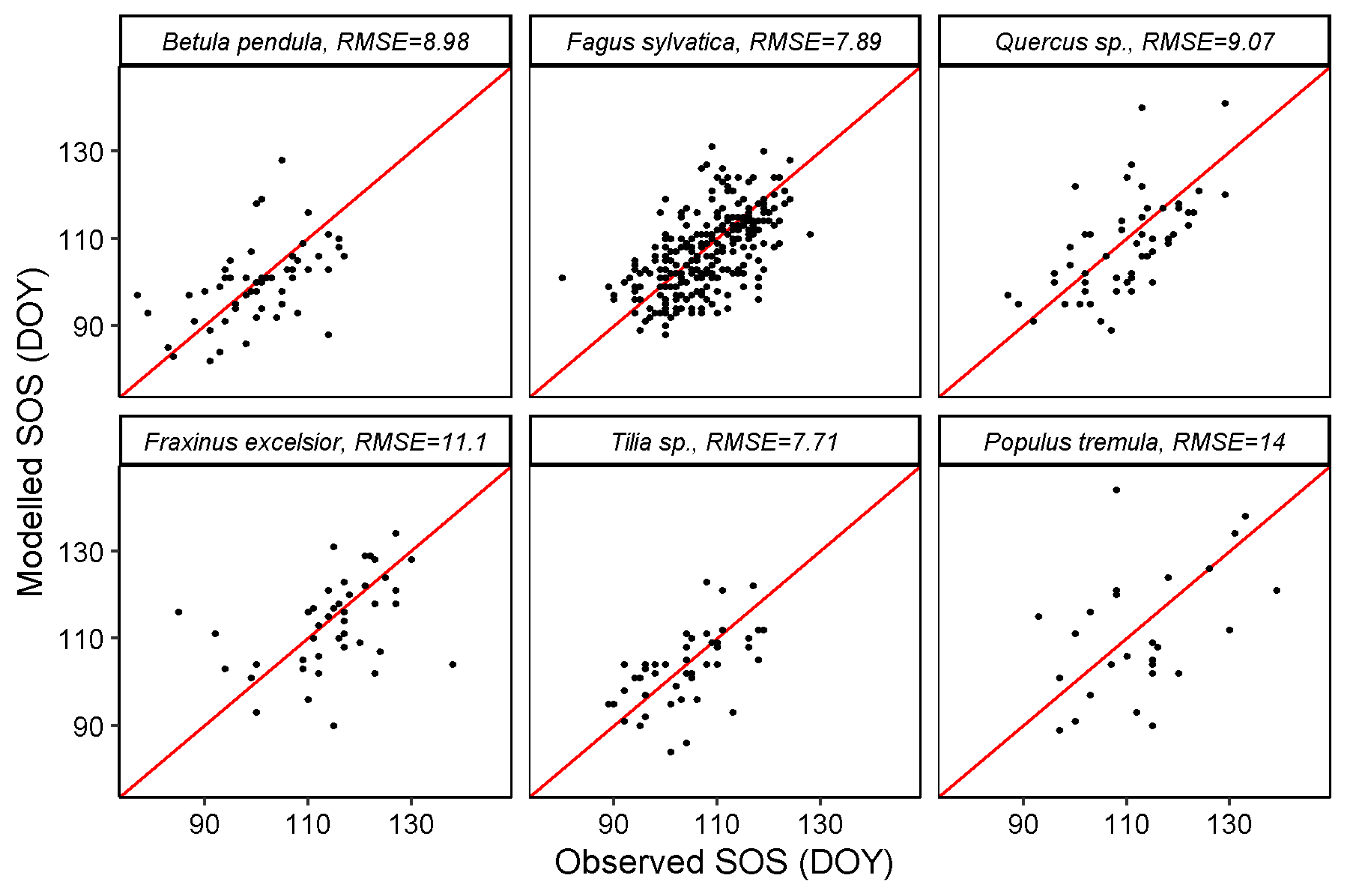
Scatter plots of modelled vs. observed SOS (Figure 7) or EOS (Figure 8) based on the holdout years (left out during training) show relatively low RMSEs in general, considering the original temporal resolution of the remote sensing data (8 days). For SOS, the lowest RMSE of 7.71 days was recorded for Tilia sp. A comparable RMSE of 7.89 days was obtained for Fagus sylvatica. The highest average RMSE recorded is 14 days for Populus tremula. The RMSEs of other species Betula pendula, Quercus sp. and Fraxinus excelsior were 8.98, 9.07 and 11.1 days, respectively.
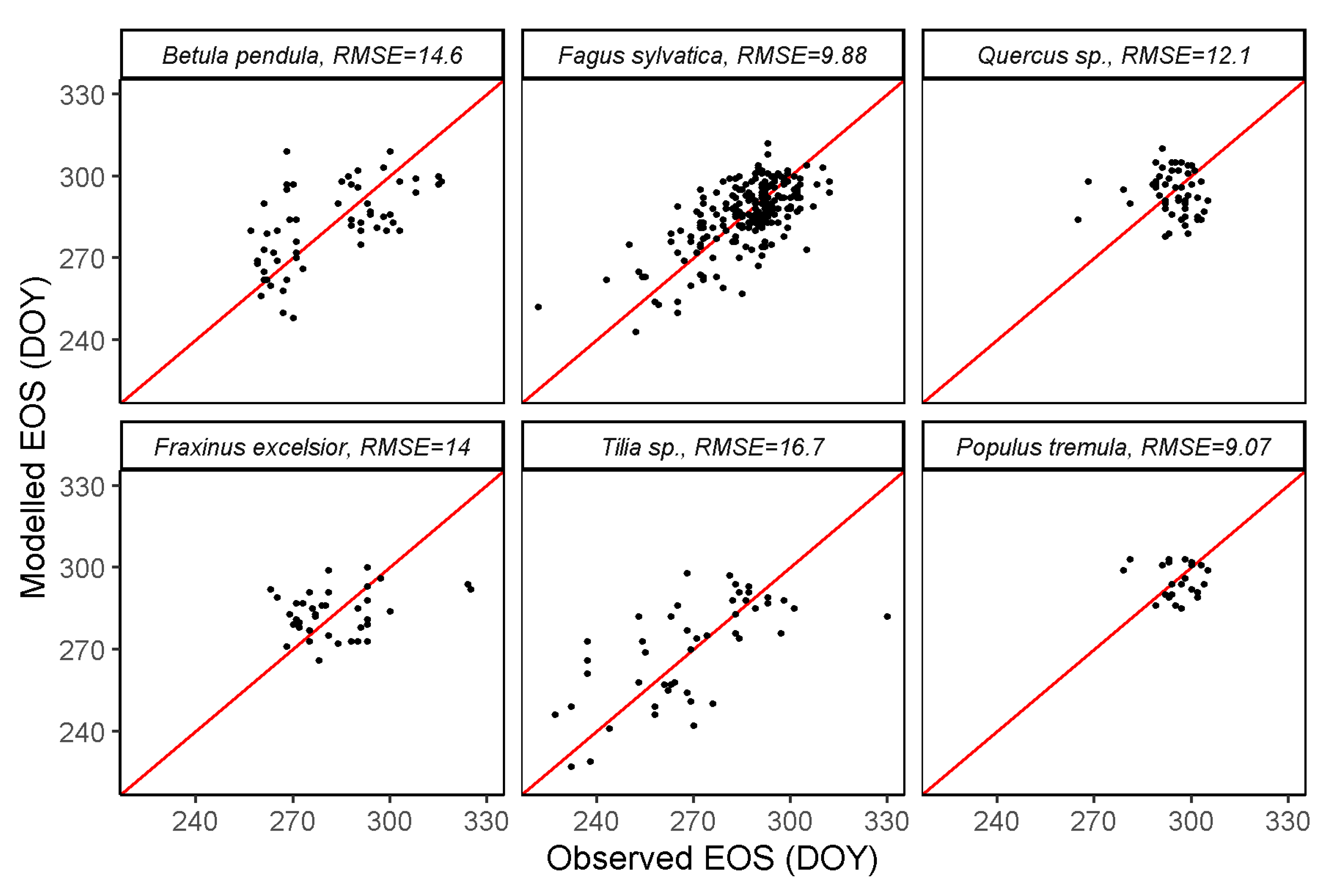
The RMSE recorded for EOS is generally greater than 10 days, with the exception of Fagus sylvatica and Populus tremula (Figure 8). While the errors for EOS are generally higher than for SOS, this was not the case for Populus tremula (9.07 days for EOS vs. 14 days for SOS).
3.3. SOS and EOS Estimates from Other Vegetation Indices
The RMSEs obtained per species for SOS and EOS are reported in Table 1. This includes RMSEs for SOS and EOS derived from MODIS GPP (Figure 7 and Figure 8), but also from MODIS LAI, EVI and NDVI as well as Landsat 7 EVI and NDVI (Figures S1–S15). The results show large differences across the different vegetation indices. While lower RMSE values were obtained for EVI compared to NDVI (both MODIS and Landsat 7), these errors as well as those obtained with MODIS LAI were much higher than those obtained from MODIS GPP data.
4. Discussion
4.1. Mixed Tree Species Forests Peculiarities
Modelling phenology from remote sensing requires reliable, dense, and frequent ground observation, which is a challenge in the case of mixed forests. In fact, observations are made on individual tree species, often selected not considering site characteristics such as the aspect and slope of the terrain, or the microclimate conditions of trees in near forests. Remote sensing pixels, however, blend together several trees and site conditions, making it difficult to relate field observations to remote sensing data [52]. A mixture of coniferous and broadleaved species is a well-studied case of the influence of mixture on phenology metrics. In fact, at the end of season in autumn, pixels with significant cover of coniferous tree species would probably lead to a slow decrease in vegetation indices as compared to pixels with pure deciduous broadleaved species, which makes the estimation of the date of EOS more uncertain, as it was the case in our study. On the other hand, a mixture of different deciduous species in the same pixel leads to more difficulties in estimating the date of SOS for individual species, due to the different timing of bud-burst for the different species [53].
The use of remote sensing to study phenology at species level requires a continuous and large mono-species area [54,55], which needs to be even larger for coarse-resolution remote sensing data such as the MODIS GPP product. This is usually resolved by finding larger pure stands in similar conditions as the observed tree [49]. This could constitute a substantial source of error in phenology modelling from remote sensing data, since the slight differences (altitude, slope, aspect) in the substitute forest stand could result in substantial discrepancies in the modelled phenology. In fact, the bioclimatic law suggests four-day offsets in phenology events for a difference of 120 m in altitudes [56], which means that the 200 m margin considered in the search of substitute stands could be an important source of error in our study. In addition, the relatively low minimum area of pure forest (1 ha) adopted in our study due to the scarcity of large pure stands of some tree species, meant low fractional cover of the species of interest in the remote sensing pixel, which is an important source of uncertainty in the model.
White et al. [53] predicted SOS with a mean absolute error of 11 days in mixed forests, 9 days in hardwood dominated forests, and 7 days in a nearly pure sugar maple forest using Landsat TM imagery. This is consistent with our study that showed a low SOS RMSE (7.89 days) for Fagus sylvatica, which represents the prevalent deciduous forest across Slovenia. The lower SOS RMSE observed for Tilia sp. (7.71 days) is probably due to the fact that Tilia species is a secondary tree species which rarely forms pure stands in Slovenia, and the few significant stands are mostly located in areas less suitable for other tree species. This, however, does not explain the high error obtained for EOS for the same tree species (16.7 days).
4.2. Challenges of the Seasonal Midpoint Method
Slovenian forests are generally situated in hilly/mountainous landscapes with high cloud cover. This means reduced cloud-free data coverage of different vegetation indices, which leads to difficulties in observing the seasonality in vegetation indices, and thus poor estimates of phenology metrics [53]. Since the SM method is based on the yearly maximum and minimum vegetation indices values as well as the trend over the year, it is very important to reconstruct the seasonal trend of the vegetation growth as reliably as possible. The smoothing algorithm or curve fitting method chosen for reconstructing continuous daily remote sensing data would greatly affect the seasonal pattern, and hence influence the results of the SM method [11,36] even more when large gaps exist in the time series. In this study, the choice of the double logistic functions is supported by the fact that it proved to describe the vegetation indices well over the growing season, by handling outliers effectively [26]. In the few years where the double logistic function failed to capture the seasonality due to a lot of missing data, for instance, the Gaussian function performed relatively well. Therefore, instead of using a single method as in most previous studies, we used the best fit between a Gaussian function and two double logistic functions for each year, in order to ensure the best fit and guarantee the lowest errors in modelled SOS and EOS.
The popularity of the SM method is due to its simplicity. Despite its good performance in modelling plant phenology, it is sensitive to several factors that could affect the seasonality reflected by satellite data. Based on the midpoint of the amplitude of one year of remote sensing vegetation indices or GPP, the SM method can be dynamically applied to each year separately, in which case it is very sensitive to partial snow and/or cloud cover, droughts, etc. of that year, introducing large variations in the results of the method. This is the reason for adopting a constant threshold over multiple years [11,57]. On the other hand, fixed threshold approaches have limitations such as a poor estimation of the phenology of some particular years, and the need to use a given threshold only for a number of years since long time series can show a positive trend in vegetation indices, leading to early SOS estimates in future [57]. Threshold methods often use a constant and the same threshold for defining SOS and EOS. The most common threshold used is 50% of the amplitude of the considered vegetation index over the season. However, Huang et al. [58] found that there is no optimal threshold that works for all plant species. In fact, the threshold for SOS (and EOS) depends on the plant species, the plant community, and the background reflectance properties at a particular site [34,59]. These support the choice of a tuned threshold for each combination of stations and species in our study, therefore offering the best possible estimates of the SM method across different situations.
4.3. Reasons for the Difficulty in Estimating Phenology from Remote Sensing
One possible source of error in phenology modelling originates from errors in observations, especially in empirical approaches as adopted in this study, where the model is developed based on observations. Visual phenological observations demand a person to observe and record the phenological phases in the field, and this approach is not free of subjective judgments and biases of an individual observer when visually assessing a canopy. Differences of up to 7 days have been found among different phenological observers. Differences are most visible when an observer is replaced at the same location [60].
The temporal resolution of vegetation indices is very important for phenology modelling, even more important than spatial resolution, especially in pure or nearly pure forests [36,61,62]. In the mixed forests of this study, this was also proven by the poor performance of Landsat-derived vegetation indices, which had a low temporal resolution of cloud- and snow-free data, despite their higher spatial resolution. The good performance of MODIS GPP is likely due to their good temporal resolution, despite a very coarse spatial resolution. However, it is worth noting that it is also the combination of both temporal and spatial resolutions, as well as the adequacy of the chosen remote sensing data that determine the performance of remote sensing-based phenology models. In fact, despite the higher temporal resolution of MODIS LAI data compared to MODIS GPP, the noise in LAI data caused a worse performance than GPP.
Events characterizing the EOS (leaf colouring and leaf fall) have been studied less than spring events of SOS (or leaf unfolding), although various authors have reported that the timing of leaf senescence shows less year-to-year variability and is concomitant with less favourable conditions for photosynthesis [63]. However, some factors influence leaf colouring, which could lead to difficulties in predicting the timing of the onset of leaf colouring for some particular years and species. In fact, Vilhar et al. [64] reported a sensitivity of the general leaf colouring of pedunculated oak to summer and autumn temperature, with higher temperatures (June–October) inducing later leaf colouring, while the leaf colouring of beech was more sensitive to spring temperature (March–May).
Autumn plant events are generally more difficult to define and are influenced by sudden individual weather events such as high winds or a single frost [65]. This makes the modelling of EOS particularly more difficult than SOS. For instance, errors of modelled EOS are usually ≥10 days, whereas usual errors in modelling SOS are around 7 days in physiological phenology models [63,66], which relates very well to the performance of the remote-sensing-based model of our study, with larger errors for EOS. The phenological phase ‘leaf colouring’ (or EOS) is more problematic to recognise than the first few green leaves in spring (SOS), because the phase definition refers to 50% of all leaves coloured, including leaves both on branches and on the ground. The variation among individual trees at comparable or identical sites is much higher than in the case of SOS [10].
In the present study, no significant effect of the fractional land share of the different groups of land use (species of interest, coniferous species, other broadleaved species, other land uses) on the best threshold of SOS was found. For EOS, however, higher values of other land uses seem to have a significant effect on the best thresholds, which fluctuate more from the usual default threshold of the SM method (0.5) with high land shares of other land uses (agriculture, grassland, bare land, buildings, etc.). In fact, agriculture and grassland mixed with a species of interest in the same remote sensing pixel would lead to more complex patterns in GPP, with a threshold not being able to capture the interannual variations of the EOS. This is supported by the findings of Klosterman et al. [67], that phenology, and in particular EOS, is more difficult to estimate using remote sensing in heterogeneous ecosystems with a low fractional cover of forests.
5. Conclusions
In this study, the SM method was applied to MODIS GPP data in order to estimate phenological events of start of season (SOS) and end of season (EOS) for six tree species in mixed forests in Slovenia for several years between 2004 and 2019. The results reinforce the importance of temporal resolution over spatial resolution in modelling tree phenology, due to the importance of seasonality, particularly for the SM method. It also appeared clearly that the usual threshold of 0.5 is not best in most cases, especially for estimating the EOS. Finally, this study showed that despite the difficulty in modelling the phenology of different tree species in a mixed forest using remote sensing, it remains possible with moderate errors. It was possible to estimate SOS and EOS with errors as low as <8 days (Fagus sylvatica and Tilia sp.) and <10 days (Fagus sylvatica and Populus tremula), respectively.
Supplementary Materials
The following are available online at https://www.mdpi.com/article/10.3390/rs13153015/s1, Figures S1–S15: similar to Figure 6, Figure 7 and Figure 8 of this article, reproduced for five vegetation indices (MODIS LAI, MODIS EVI, MODIS NDVI, Landsat 7 EVI, and Landsat 7 NDVI).
Author Contributions
Conceptualisation, K.D.N. and U.V.; methodology, K.D.N. and U.V.; software, K.D.N.; validation, K.D.N., G.O., A.Ž. and U.V.; formal analysis, K.D.N.; investigation, G.O. and A.Ž.; resources, U.V.; data curation, G.O. and K.D.N.; writing—original draft preparation, K.D.N.; writing—review and editing, K.D.N., G.O., A.Ž. and U.V.; visualisation, K.D.N.; supervision, U.V.; project administration, U.V.; funding acquisition, U.V. All authors have read and agreed to the published version of the manuscript.
Funding
This research was funded by the Slovenian Research Agency within the core funding for the Program Group “Forest biology, ecology and technology”, grant number P4–0107 and the FORGENIUS project that has received funding from the European Union’s Horizon 2020 research and innovation program, grant number 862221. The APC was funded by the FORGENIUS project.
Data Availability Statement
The data presented in this study are openly available in FigShare at https://doi.org/10.6084/m9.figshare.14829081.v1, reference number 14829081, accessed on 30 July 2021.
Conflicts of Interest
The authors declare that no conflict of interest exists.
References
- Matongera, T.N.; Mutanga, O.; Sibanda, M.; Odindi, J. Estimating and Monitoring Land Surface Phenology in Rangelands: A Review of Progress and Challenges. Remote Sens. 2021, 13, 2060. [Google Scholar] [CrossRef]
- Koch, E.; Bruns, E.; Chmielewski, F.M.; Defila, C.; Lipa, W.; Menzel, A.; Baddour, O.; Kontongomde, H. World Climate Data and Monitoring Programme; WMO: Geneva, Switzerland, 2009. [Google Scholar]
- Donnelly, A.; Caffarra, A.; O’Neill, B.F. A review of climate-driven mismatches between interdependent phenophases in terrestrial and aquatic ecosystems. Int. J. Biometeorol. 2011, 55, 805–817. [Google Scholar] [CrossRef]
- Menzel, A.; Sparks, T.H.; Estrella, N.; Koch, E.; Aasa, A.; Ahas, R.; Alm-Kübler, K.; Bissolli, P.; Braslavská, O.; Briede, A.; et al. European phenological response to climate change matches the warming pattern. Glob. Chang. Biol. 2006, 12, 1969–1976. [Google Scholar] [CrossRef]
- Doi, H.; Katano, I. Phenological timings of leaf budburst with climate change in Japan. Agric. For. Meteorol. 2008, 148, 512–516. [Google Scholar] [CrossRef]
- Chen, X.; Xu, L. Temperature controls on the spatial pattern of tree phenology in China’s temperate zone. Agric. For. Meteorol. 2012, 154–155, 195. [Google Scholar] [CrossRef]
- Davi, H.; Dufrêne, E.; Francois, C.; Le Maire, G.; Loustau, D.; Bosc, A.; Rambal, S.; Granier, A.; Moors, E. Sensitivity of water and carbon fluxes to climate changes from 1960 to 2100 in European forest ecosystems. Agric. For. Meteorol. 2006, 141, 35–56. [Google Scholar] [CrossRef]
- Piao, S.; Friedlingstein, P.; Ciais, P.; Viovy, N.; Demarty, J. Growing season extension and its impact on terrestrial carbon cycle in the Northern Hemisphere over the past 2 decades. Glob. Biogeochem. Cycles 2007, 21, 21. [Google Scholar] [CrossRef]
- Koch, E.; Bruns, E.; Chmielewski, F.-M.; Defila, C.; Lipa, W.; Menzel, A. Guidelines for Phenological Observations; WMO: Geneva, Switzerland, 2007. [Google Scholar]
- Vilhar, U.; De Groot, M.; Žust, A.; Skudnik, M.; Simončič, P. Predicting phenology of European beech in forest habitats. iForest Biogeosci. For. 2018, 11, 41–47. [Google Scholar] [CrossRef] [Green Version]
- Studer, S.; Stöckli, R.; Appenzeller, C.; Vidale, P.L. A comparative study of satellite and ground-based phenology. Int. J. Biometeorol. 2007, 51, 405–414. [Google Scholar] [CrossRef] [PubMed] [Green Version]
- Ge, Q.; Dai, J.; Cui, H.; Wang, H. Spatiotemporal variability in start and end of growing season in China related to climate variability. Remote Sens. 2016, 8, 16. [Google Scholar] [CrossRef] [Green Version]
- Reed, B.C.; White, M.; Brown, J.F. Remote Sensing Phenology. In Phenology: An Integrative Environmental Science; Schwartz, M.D., Ed.; Springer: Dordrecht, The Netherlands, 2003; ISBN 978-94-007-0632-3. [Google Scholar]
- Zuo, L.; Liu, R.; Liu, Y.; Shang, R. Effect of Mathematical Expression of Vegetation Indices on the Estimation of Phenology Trends from Satellite Data. Chin. Geogr. Sci. 2019, 29, 756–767. [Google Scholar] [CrossRef] [Green Version]
- Brown, L.A.; Dash, J.; Ogutu, B.O.; Richardson, A.D. On the relationship between continuous measures of canopy greenness derived using near-surface remote sensing and satellite-derived vegetation products. Agric. For. Meteorol. 2017, 247, 280–292. [Google Scholar] [CrossRef] [Green Version]
- Tan, B.; Gao, F.; Wolfe, R.E.; Pedelty, J.A.; Nightingale, J.; Morisette, J.T.; Ederer, G.A. An Enhanced TIMESAT Algorithm for Estimating Vegetation Phenology Metrics From MODIS Data. IEEE J. Sel. Top. Appl. Earth Obs. Remote Sens. 2011, 4, 361–371. [Google Scholar] [CrossRef]
- Zhang, X.; Liu, L.; Liu, Y.; Jayavelu, S.; Wang, J.; Moon, M.; Henebry, G.M.; Friedl, M.A.; Schaaf, C.B. Generation and evaluation of the VIIRS land surface phenology product. Remote Sens. Environ. 2018, 216, 212–229. [Google Scholar] [CrossRef]
- Gonsamo, A.; Chen, J.M.; D’Odorico, P. Deriving land surface phenology indicators from CO2 eddy covariance measurements. Ecol. Indic. 2013, 29, 203–207. [Google Scholar] [CrossRef]
- Gonsamo, A.; Chen, J.M.; David, T.P.; Kurz, W.A.; Wu, C. Land surface phenology from optical satellite measurement and CO2 eddy covariance technique. J. Geophys. Res. Biogeosci. 2012, 117, 3032. [Google Scholar] [CrossRef]
- Bórnez, K.; Descals, A.; Verger, A.; Peñuelas, J. Land surface phenology from VEGETATION and PROBA-V data. Assessment over deciduous forests. Int. J. Appl. Earth Obs. Geoinf. 2020, 84, 101974. [Google Scholar] [CrossRef]
- Kandasamy, S.; Baret, F.; Verger, A.; Neveux, P.; Weiss, M. A comparison of methods for smoothing and gap filling time series of remote sensing observations – application to MODIS LAI products. Biogeosciences 2013, 10, 4055–4071. [Google Scholar] [CrossRef] [Green Version]
- Zhao, H.; Yang, Z.; Di, L.; Pei, Z. Evaluation of Temporal Resolution Effect in Remote Sensing Based Crop Phenology Detection Studies, Proceedings of the IFIP Advances in Information and Communication Technology, Surat, India, 21–25 May 2012; Springer: Berlin/Heidelberg, Germany, 2012; Volume 369 AICT. [Google Scholar]
- Zhang, X.; Friedl, M.A.; Schaaf, C.B.; Strahler, A.H.; Hodges, J.C.F.; Gao, F.; Reed, B.C.; Huete, A. Monitoring vegetation phenology using MODIS. Remote Sens. Environ. 2003, 84, 471–475. [Google Scholar] [CrossRef]
- Cao, R.; Chen, J.; Shen, M.; Tang, Y. An improved logistic method for detecting spring vegetation phenology in grasslands from MODIS EVI time-series data. Agric. For. Meteorol. 2015, 200, 9–20. [Google Scholar] [CrossRef]
- Elmore, A.J.; Guinn, S.M.; Minsley, B.J.; Richardson, A.D. Landscape controls on the timing of spring, autumn, and growing season length in mid-Atlantic forests. Glob. Chang. Biol. 2012, 18, 656–674. [Google Scholar] [CrossRef] [Green Version]
- Beck, P.S.A.; Atzberger, C.; Høgda, K.A.; Johansen, B.; Skidmore, A.K. Improved monitoring of vegetation dynamics at very high latitudes: A new method using MODIS NDVI. Remote Sens. Environ. 2006, 100, 321–334. [Google Scholar] [CrossRef]
- Jönsson, P.; Eklundh, L. Seasonality extraction by function fitting to time-series of satellite sensor data. IEEE Trans. Geosci. Remote Sens. 2002, 40, 1824–1832. [Google Scholar] [CrossRef]
- De Beurs, K.M.; Henebry, G.M. Land surface phenology, climatic variation, and institutional change: Analyzing agricultural land cover change in Kazakhstan. Remote Sens. Environ. 2004, 89, 497–509. [Google Scholar] [CrossRef]
- De Beurs, K.M.; Henebry, G.M. Land surface phenology and temperature variation in the International Geosphere-Biosphere Program high-latitude transects. Glob. Chang. Biol. 2005, 11, 779–790. [Google Scholar] [CrossRef]
- Chen, J.; Jönsson, P.; Tamura, M.; Gu, Z.; Matsushita, B.; Eklundh, L. A simple method for reconstructing a high-quality NDVI time-series data set based on the Savitzky-Golay filter. Remote Sens. Environ. 2004, 91, 332–344. [Google Scholar] [CrossRef]
- Piao, S.; Fang, J.; Zhou, L.; Ciais, P.; Zhu, B. Variations in satellite-derived phenology in China’s temperate vegetation. Glob. Chang. Biol. 2006, 12, 672–685. [Google Scholar] [CrossRef]
- Belda, S.; Pipia, L.; Morcillo-Pallarés, P.; Rivera-Caicedo, J.P.; Amin, E.; De Grave, C.; Verrelst, J. DATimeS: A machine learning time series GUI toolbox for gap-filling and vegetation phenology trends detection. Environ. Model. Softw. 2020, 127, 104666. [Google Scholar] [CrossRef]
- Dronova, I.; Taddeo, S.; Hemes, K.S.; Knox, S.H.; Valach, A.; Oikawa, P.Y.; Kasak, K.; Baldocchi, D.D. Remotely sensed phenological heterogeneity of restored wetlands: Linking vegetation structure and function. Agric. For. Meteorol. 2021, 296. [Google Scholar] [CrossRef]
- Reed, B.C.; Brown, J.F.; VanderZee, D.; Loveland, T.R.; Merchant, J.W.; Ohlen, D.O. Measuring phenological variability from satellite imagery. J. Veg. Sci. 1994, 5, 703–714. [Google Scholar] [CrossRef]
- Xu, H.; Twine, T.; Yang, X. Evaluating Remotely Sensed Phenological Metrics in a Dynamic Ecosystem Model. Remote Sens. 2014, 6, 4660–4686. [Google Scholar] [CrossRef] [Green Version]
- White, M.A.; De Beurs, K.M.; Didan, K.; Inouye, D.W.; Richardson, A.D.; Jensen, O.P.; O’keefe, J.; Zhang, G.; Nemani, R.R.; Van Leeuwen, W.J.D.; et al. Intercomparison, interpretation, and assessment of spring phenology in North America estimated from remote sensing for 1982–2006. Glob. Chang. Biol. 2009, 15, 2335–2359. [Google Scholar] [CrossRef]
- Wang, H.; Dai, J.; Ge, Q. Comparison of satellite and ground-based phenology in China’s temperate monsoon area. Adv. Meteorol. 2014, 2014, 10. [Google Scholar] [CrossRef]
- Liang, L.; Schwartz, M.D.; Fei, S. Validating satellite phenology through intensive ground observation and landscape scaling in a mixed seasonal forest. Remote Sens. Environ. 2011, 115, 143–157. [Google Scholar] [CrossRef]
- Melaas, E.K.; Friedl, M.A.; Zhu, Z. Detecting interannual variation in deciduous broadleaf forest phenology using Landsat TM/ETM+ data. Remote Sens. Environ. 2013, 132, 176–185. [Google Scholar] [CrossRef]
- Liu, L.; Liang, L.; Schwartz, M.D.; Donnelly, A.; Wang, Z.; Schaaf, C.B.; Liu, L. Evaluating the potential of MODIS satellite data to track temporal dynamics of autumn phenology in a temperate mixed forest. Remote Sens. Environ. 2015, 160, 156–165. [Google Scholar] [CrossRef]
- Moon, M.; Zhang, X.; Henebry, G.M.; Liu, L.; Gray, J.M.; Melaas, E.K.; Friedl, M.A. Long-term continuity in land surface phenology measurements: A comparative assessment of the MODIS land cover dynamics and VIIRS land surface phenology products. Remote Sens. Environ. 2019, 226, 74–92. [Google Scholar] [CrossRef]
- Misra, G.; Asam, S.; Menzel, A. Ground and satellite phenology in alpine forests are becoming more heterogeneous across higher elevations with warming. Agric. For. Meteorol. 2021, 303, 108383. [Google Scholar] [CrossRef]
- Čufar, K.; de Luis, M.; Saz, M.A.; Črepinšek, Z.; Kajfež-Bogataj, L. Temporal shifts in leaf phenology of beech (Fagus sylvatica) depend on elevation. Trees Struct. Funct. 2012, 26, 1091–1100. [Google Scholar] [CrossRef]
- De Luis, M.; Čufar, K.; Saz, M.A.; Longares, L.A.; Ceglar, A.; Kajfež-Bogataj, L. Trends in seasonal precipitation and temperature in Slovenia during 1951–2007. Reg. Environ. Chang. 2014, 14, 1801–1810. [Google Scholar] [CrossRef]
- Kermavnar, J.; Kutnar, L. Patterns of Understory Community Assembly and Plant Trait-Environment Relationships in Temperate SE European Forests. Diversity 2020, 12, 91. [Google Scholar] [CrossRef] [Green Version]
- Žust, A. Fenologija v Sloveniji: Priročnik za Fenološka Opazovanja [Phenology in Slovenia: Manual for Phenological Observations]; Ministrstvo za okolje in prostor: Ljubljana, Slovenia, 2015. [Google Scholar]
- Meier, U. Phenological Growth Stages. In An Integrative Environmental Science. Tasks for Vegetation Science; Schwartz, M.D., Ed.; Springer: Dordrecht, The Netherlands, 2003; Volume 39, pp. 269–283. [Google Scholar]
- Slovenian Forest Service Forest Stands Map. Available online: http://www.zgs.si/eng/slovenian_forests/forests_in_slovenia/maps/index.html (accessed on 4 June 2021).
- Rodriguez-Galiano, V.F.; Dash, J.; Atkinson, P.M. Intercomparison of satellite sensor land surface phenology and ground phenology in Europe. Geophys. Res. Lett. 2015, 42, 2253–2260. [Google Scholar] [CrossRef] [Green Version]
- Mann, H.B.; Whitney, D.R. On a Test of Whether one of Two Random Variables is Stochastically Larger than the Other. Ann. Math. Stat. 1947, 18, 50–60. [Google Scholar] [CrossRef]
- Hinton, P.R. Mann–Whitney U Test. In Encyclopedia of Research Design; Salkind, N., Ed.; SAGE Publications, Inc.: Thousand Oaks, CA, USA, 2010; pp. 748–750. ISBN 9781412961288. [Google Scholar]
- Henebry, G.M.; De Beurs, K.M. Remote sensing of land surface phenology: A prospectus. In Phenology: An Integrative Environmental Science; Schwartz, M., Ed.; Springer: Dordrecht, The Netherlands, 2013; pp. 385–411. ISBN 9789400769250. [Google Scholar]
- White, K.; Pontius, J.; Schaberg, P. Remote sensing of spring phenology in northeastern forests: A comparison of methods, field metrics and sources of uncertainty. Remote Sens. Environ. 2014, 148, 97–107. [Google Scholar] [CrossRef]
- Fawcett, D.; Bennie, J.; Anderson, K. Monitoring spring phenology of individual tree crowns using drone-acquired NDVI data. Remote Sens. Ecol. Conserv. 2020, 1–18. [Google Scholar] [CrossRef]
- Zeng, L.; Wardlow, B.D.; Xiang, D.; Hu, S.; Li, D. A review of vegetation phenological metrics extraction using time-series, multispectral satellite data. Remote Sens. Environ. 2020, 237, 111511. [Google Scholar] [CrossRef]
- Hopkins, A.D. The Bioclimatic Law. J. Washingt. Acad. Sci. 1920, 10, 34–40. [Google Scholar]
- Schwartz, M.D.; Reed, B.C.; White, M.A. Assesing satellite-derived start-of-season measures in the conterminous USA. Int. J. Climatol. 2002, 22, 1793–1805. [Google Scholar] [CrossRef]
- Huang, X.; Liu, J.; Zhu, W.; Atzberger, C.; Liu, Q. The optimal threshold and vegetation index time series for retrieving crop phenology based on a modified dynamic threshold method. Remote Sens. 2019, 11, 2725. [Google Scholar] [CrossRef] [Green Version]
- Hanes, J.M.; Liang, L.; Morisette, J.T. Land Surface Phenology. In Biophysical Applications of Satellite Remote Sensing; Hanes, J.M., Ed.; Springer Remote Sensing/Photogrammetry; Springer: Berlin/Heidelberg, Germany, 2014; pp. 99–125. ISBN 978-3-642-25046-0. [Google Scholar]
- Courter, J.R.; Johnson, R.J.; Stuyck, C.M.; Lang, B.A.; Kaiser, E.W. Weekend bias in Citizen Science data reporting: Implications for phenology studies. Int. J. Biometeorol. 2013, 57, 715–720. [Google Scholar] [CrossRef] [PubMed]
- Zhang, X.; Friedl, M.A.; Schaaf, C.B. Sensitivity of vegetation phenology detection to the temporal resolution of satellite data. Int. J. Remote Sens. 2009, 30, 2061–2074. [Google Scholar] [CrossRef]
- Cui, T.; Martz, L.; Zhao, L.; Guo, X. Investigating the impact of the temporal resolution of MODIS data on measured phenology in the prairie grasslands. GISci. Remote Sens. 2020, 57, 395–410. [Google Scholar] [CrossRef]
- Delpierre, N.; Dufrêne, E.; Soudani, K.; Ulrich, E.; Cecchini, S.; Boé, J.; François, C. Modelling interannual and spatial variability of leaf senescence for three deciduous tree species in France. Agric. For. Meteorol. 2009, 149, 938–948. [Google Scholar] [CrossRef]
- Vilhar, U.; Skudnik, M.; Ferlan, M.; Simončič, P. Influence of meteorological conditions and crown defoliation on tree phenology in intensive forest monitoring plots in Slovenia. Acta Silvae Ligni 2014, 105, 1–15. [Google Scholar] [CrossRef] [Green Version]
- Sparks, T.H.; Menzel, A. Observed changes in seasons: An overview. Int. J. Climatol. 2002, 22, 1715–1725. [Google Scholar] [CrossRef]
- Schaber, J.; Badeck, F.W. Physiology-based phenology models for forest tree species in Germany. Int. J. Biometeorol. 2003, 47, 193–201. [Google Scholar] [CrossRef] [PubMed]
- Klosterman, S.T.; Hufkens, K.; Gray, J.M.; Melaas, E.; Sonnentag, O.; Lavine, I.; Mitchell, L.; Norman, R.; Friedl, M.A.; Richardson, A.D. Evaluating remote sensing of deciduous forest phenology at multiple spatial scales using PhenoCam imagery. Biogeosciences 2014, 11, 4305–4320. [Google Scholar] [CrossRef] [Green Version]
Figure 1.
Phenological stations of the Slovenian National Phenological Network (NPN) of the Slovenian Environment Agency. The stations represented are only a subset of stations with observations of nine years or more for at least one of the tree species of interest.
Figure 1.
Phenological stations of the Slovenian National Phenological Network (NPN) of the Slovenian Environment Agency. The stations represented are only a subset of stations with observations of nine years or more for at least one of the tree species of interest.

Figure 2.
Routine for generating remote sensing pixel centre from observation stations (a tree at a given location).
Figure 2.
Routine for generating remote sensing pixel centre from observation stations (a tree at a given location).

Figure 3.
Example of one-year series of MODIS GPP data (Fagus sylvatica at Bohinjska for year 2015). Grey dots are the 8-day average for the MODIS GPP 500 m pixel, the red line is the fitted line, a is the amplitude, SOS and EOS represent the start of season and end of season, respectively, determined using the traditional SM method.

Figure 4.
Best thresholds for SOS (top panel) and EOS (bottom panel) for each combination of station and species.
Figure 4.
Best thresholds for SOS (top panel) and EOS (bottom panel) for each combination of station and species.

Figure 5.
Mann–Whitney test for comparing the share of different land uses for two groups of best thresholds (~0.5, i.e., 0.45 to 0.55, and ≠0.5, i.e., <0.45 or >0.55) at the substitute forests for SOS (A) and for EOS (B). “ns” and “*” mean non-significant (p-value ≥ 0.05) and significant (p-value < 0.05) difference, respectively.

Figure 6.
Error (modelled—observed) of SOS and EOS per station, all species and each species separately.
Figure 6.
Error (modelled—observed) of SOS and EOS per station, all species and each species separately.

Figure 7.
Modelled vs. observed SOS per species, all stations together. The red lines are identity (1:1) lines for each panel.
Figure 7.
Modelled vs. observed SOS per species, all stations together. The red lines are identity (1:1) lines for each panel.

Figure 8.
Modelled vs. observed EOS per species, all stations together. The red lines are identity (1:1) lines for each panel.
Figure 8.
Modelled vs. observed EOS per species, all stations together. The red lines are identity (1:1) lines for each panel.


Table 1.
RMSE of estimated SOS and EOS during a leave-one-out cross-validation, using different vegetation indices.
Table 1.
RMSE of estimated SOS and EOS during a leave-one-out cross-validation, using different vegetation indices.
| SOS RMSE | EOS RMSE | |||||||||||
|---|---|---|---|---|---|---|---|---|---|---|---|---|
| BP * | FS | Qs. | FE | Ts. | PT | BP | FS | Qs. | FE | Ts. | PT | |
| MODIS GPP | 8.98 | 7.89 | 9.07 | 11.1 | 7.71 | 14 | 14.6 | 9.88 | 12.1 | 14 | 16.7 | 9.07 |
| MODIS LAI | 19.4 | 26.4 | 35.7 | 24.6 | 22.4 | 29.9 | 20 | 23.5 | 23.2 | 23.8 | 17.8 | 42.6 |
| MODIS EVI | 18.1 | 15.7 | 19.1 | 14.6 | 19 | 14.9 | 16.1 | 12.6 | 14.4 | 16.6 | 19.1 | 9.21 |
| MODIS NDVI | 20.7 | 16.1 | 16 | 19.7 | 22.8 | 19.2 | 20.9 | 13 | 14.8 | 18.2 | 19.1 | 11.4 |
| Landsat 7 EVI | 26.3 | 26.9 | 28.4 | 19.7 | 19.4 | 22.9 | 25 | 23.7 | 21.5 | 17.5 | 21.4 | 18.9 |
| Landsat 7 NDVI | 35.2 | 30 | 36 | 27.3 | 26.1 | 30.6 | 25.7 | 33.4 | 27.4 | 33.5 | 27.5 | 30 |
* BP, FS, Qs., FE, Ts. and PT are the different tree species, i.e., Betula pendula, Fagus sylvatica, Quercus sp., Fraxinus excelsior, Tilia sp. and Populus tremula, respectively.
Publisher’s Note: MDPI stays neutral with regard to jurisdictional claims in published maps and institutional affiliations. |
© 2021 by the authors. Licensee MDPI, Basel, Switzerland. This article is an open access article distributed under the terms and conditions of the Creative Commons Attribution (CC BY) license (https://creativecommons.org/licenses/by/4.0/).
Share and Cite
MDPI and ACS Style
Noumonvi, K.D.; Oblišar, G.; Žust, A.; Vilhar, U. Empirical Approach for Modelling Tree Phenology in Mixed Forests Using Remote Sensing. Remote Sens. 2021, 13, 3015. https://doi.org/10.3390/rs13153015
AMA Style
Noumonvi KD, Oblišar G, Žust A, Vilhar U. Empirical Approach for Modelling Tree Phenology in Mixed Forests Using Remote Sensing. Remote Sensing. 2021; 13(15):3015. https://doi.org/10.3390/rs13153015
Chicago/Turabian StyleNoumonvi, Koffi Dodji, Gal Oblišar, Ana Žust, and Urša Vilhar. 2021. "Empirical Approach for Modelling Tree Phenology in Mixed Forests Using Remote Sensing" Remote Sensing 13, no. 15: 3015. https://doi.org/10.3390/rs13153015
Note that from the first issue of 2016, this journal uses article numbers instead of page numbers. See further details here.