Article

Evaluating WorldClim Version 1 (1961–1990) as the Baseline for Sustainable Use of Forest and Environmental Resources in a Changing Climate

1
CREA—Research Centre for Forestry and Wood, I-52100 Arezzo, Italy
2
Slovenian Forestry Institute, Vecna pot 2, 1000 Ljubljana, Slovenia
3
European Forest Institute, 53113 Bonn, Germany
*
Author to whom correspondence should be addressed.
Sustainability 2019, 11(11), 3043; https://doi.org/10.3390/su11113043
Submission received: 29 April 2019 / Revised: 23 May 2019 / Accepted: 27 May 2019 / Published: 29 May 2019
(This article belongs to the Special Issue Forest Biodiversity, Conservation and Sustainability)

Abstract

:
WorldClim version 1 is a high-resolution, global climate gridded dataset covering 1961–1990; a “normal” climate. It has been widely used for ecological studies thanks to its free availability and global coverage. This study aims to evaluate the quality of WorldClim data by quantifying any discrepancies by comparison with an independent dataset of measured temperature and precipitation records across Europe. BIO1 (mean annual temperature, MAT) and BIO12 (mean total annual precipitation, MAP) were used as proxies to evaluate the spatial accuracy of the WorldClim grids. While good representativeness was detected for MAT, the study demonstrated a bias with respect to MAP. The average difference between WorldClim predictions and climate observations was around +0.2 °C for MAT and −48.7 mm for MAP, with large variability. The regression analysis revealed a good correlation and adequate proportion of explained variance for MAT (adjusted R2 = 0.856) but results for MAP were poor, with just 64% of the variance explained (adjusted R2 = 0.642). Moreover no spatial structure was found across Europe, nor any statistical relationship with elevation, latitude, or longitude, the environmental predictors used to generate climate surfaces. A detectable spatial autocorrelation was only detectable for the two most thoroughly sampled countries (Germany and Sweden). Although further adjustments might be evaluated by means of geostatistical methods (i.e., kriging), the huge environmental variability of the European environment deeply stressed the WorldClim database. Overall, these results show the importance of an adequate spatial structure of meteorological stations as fundamental to improve the reliability of climate surfaces and derived products of the research (i.e., statistical models, future projections).

1. Introduction

Easy access to standardized climate data with global coverage is paramount for the advancement of many ecological studies and to understand future ecosystem services provided by forest systems [1,2,3] and productive lands in agriculture [4,5]. One of the main aims for researchers dealing with environmental resources has become to forecast possible impacts of climate change on organisms and to evaluate possible mitigation [6,7,8,9]. In the past few decades, many conservation strategies have been suggested in order to maintain human well-being and ensure an adequate level of welfare [10] from (relatively) simple management strategies [4,11], including “assisted migration” [12,13,14], a controversial protocol that includes translocating more adapted or resilient genotypes for conservation or to improve the resilience of ecosystems. Such efforts are often driven by statistical models [14,15,16,17] and management simulators [18,19], with both genetic variation and phenotypic plasticity included in the statistical models as covariates [20,21,22]. However, despite modelling efforts, such studies always require absolutely reliable climate data to be used as both baseline (e.g., 30-year average climate data) and for future predictions. Furthermore, while the uncertainty around GCMs and future trajectories is well known [23,24,25], information on current ecological limits of forest tree species has also been questioned [26]. In this context, the interest of researchers in gridded climate datasets has grown strongly.
The interpolation method, the spatial resolution and the coverage are the three main features that researchers use to select the most suitable datasets for their research [27,28,29,30]. The first release of the WorldClim dataset [31] is probably the most famous gridded climate dataset, widely used for ecological studies and freely available from (www.worldclim.org). Thanks to its high resolution (30 arc-second in the WGS84 reference system and approximately 1 km at the equator), global coverage, and availability, it has been used and cited more than 5200 times since publication [31]. The dataset is suitable for basic and applied studies in ecology, including forestry and ecological modeling [32,33,34], as well as to construct related datasets such as bio-geographical zones or environmental stratifications [35]. One of the main products of this database is “version 1”, representative of the 1961–1990 climate normal period for the whole globe, including Antarctica. This version 1 dataset was generated by interpolating weather station data with the ANUSPLIN software (version 4.3) using latitude, longitude, and elevation as independent variables. The software implements a thin-plate smoothing spline procedure, using every station as a data point. A second-order spline function was fitted by the Authors using the above three variables, which produced the lowest overall cross-validation errors [31]. Considering the ANUSPLIN program creates a continuous surface projection, the LAPGRD program was used to create a global grid of climate surfaces with 30 arc-seconds horizontal and vertical resolution commonly referred to as 1 km2 resolution. Raster maps for monthly precipitation amount and mean, maximum, and minimum air temperature were then provided. Raw data came from weather stations retrieved from various databases including GHCN, WMO climatological normals, FAOCLIM 2.0, CIAT, and regional databases and, where possible, restricted to the period 1950–2000. Quality control measures were taken to remove duplicate records, giving precedence to the GHCN database. After the quality control check and cleaning, the database consisted of precipitation records from 47,554 locations and mean air temperature from 24,542 locations [31]. Then elevation bias in weather stations was related to latitude and presence of mountain ranges. However, local records from many European countries were not easily accessible and WorldClim climate surfaces for Europe were constructed using 1263 records for air temperature and 2116 for precipitation.
WorldClim version 1 has recently been acknowledged to be representative of the 1961–1990 climate normal period. This time-slice has been widely used as the pre-industrial climate in many papers about the potential impact of climate change on ecosystems [1,3,26,28,36,37] and other ecological fields. Nevertheless, given the detailed description provided by the Authors in their paper, the question remains whether the quality of the WorldClim climate surfaces as a proxy of the climate baseline is adequate in complex environments such as, for instance, the European environment.
The present study aims to assess and quantify the reliability of WorldClim climate raster maps for Europe. We compared WorldClim with observed average values for mean annual temperature and total annual precipitation for the period 1961–1990. Data were retrieved for the whole of Europe building an independent dataset with data from many meteorological services. Then statistical analysis was run in order to evaluate the reliability of this dataset across the study area.

2. Materials and Methods

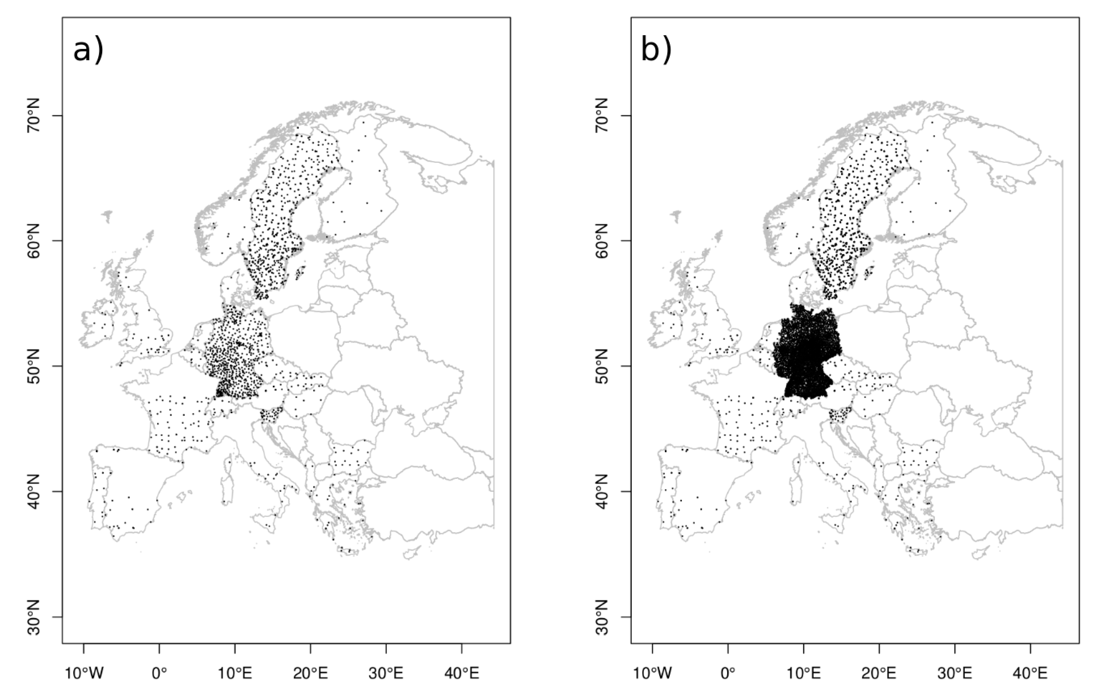
2.1. Construction and Description of the Database Used for Comparison

To investigate WorldClim’s reliability in predicting baseline climate conditions we compiled an independent climate dataset by collecting data from weather services across Europe which were already freely available or delivered upon request (Table 1). All data were specifically requested or downloaded as monthly averaged values over the 30-year normal period (1961–1990). Local monthly air temperature averages (MAT) and precipitation sums (MAP) were aggregated to calculate annual values. In total we retrieved data from 6659 meteostations across Europe, with 1759 records for temperature and 6526 records for precipitation (Figure 1). Most of the records were retrieved for Germany and Sweden with 4825 and 1391 meteostations, respectively, while for some countries, records were much fewer (e.g., Spain, France, Italy) or totally absent (e.g., Serbia, Poland, Romania).
Nevertheless, even if not equally distributed geographically, neither balanced concerning the ecological regions of Europe, we considered the distribution of the collected data as adequate for the purpose. Despite the lack of uniform coverage of both geography and ecological regions, we considered the data collected to be adequate for subsequent analysis.
Moreover we tested the random distribution of MAT and MAP with the randtest package of the R statistical language [38]. The database was carefully checked and cleaned to remove entries with missing data and to geo-reference each record. Very few points (112), corresponding to less than 1% of all the records, lay outside country borders or land masses due to coordinate uncertainties, which reflects the high-quality of the new database. Such records were removed completely from the database in order to avoid any influences on the calculations.

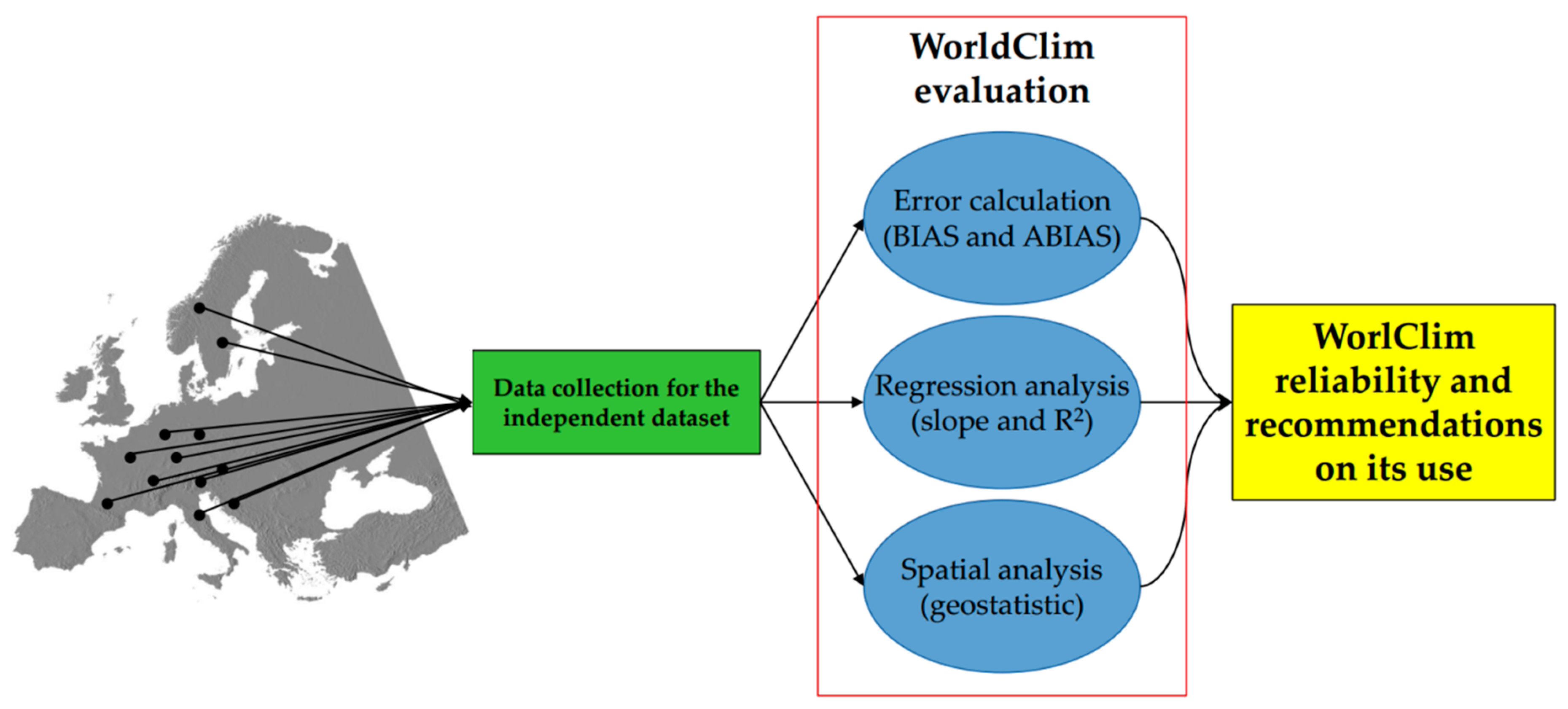
2.2. Comparisons and Statistical Procedures
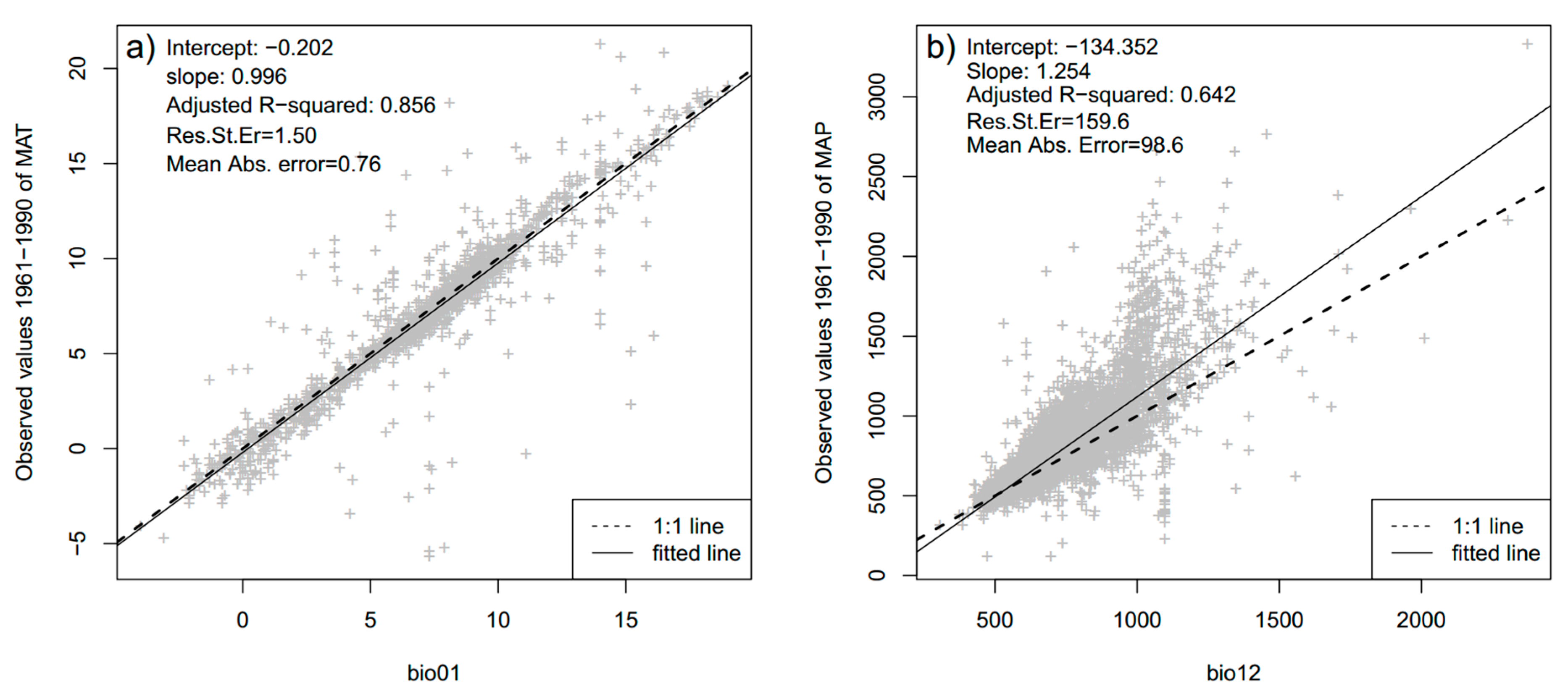
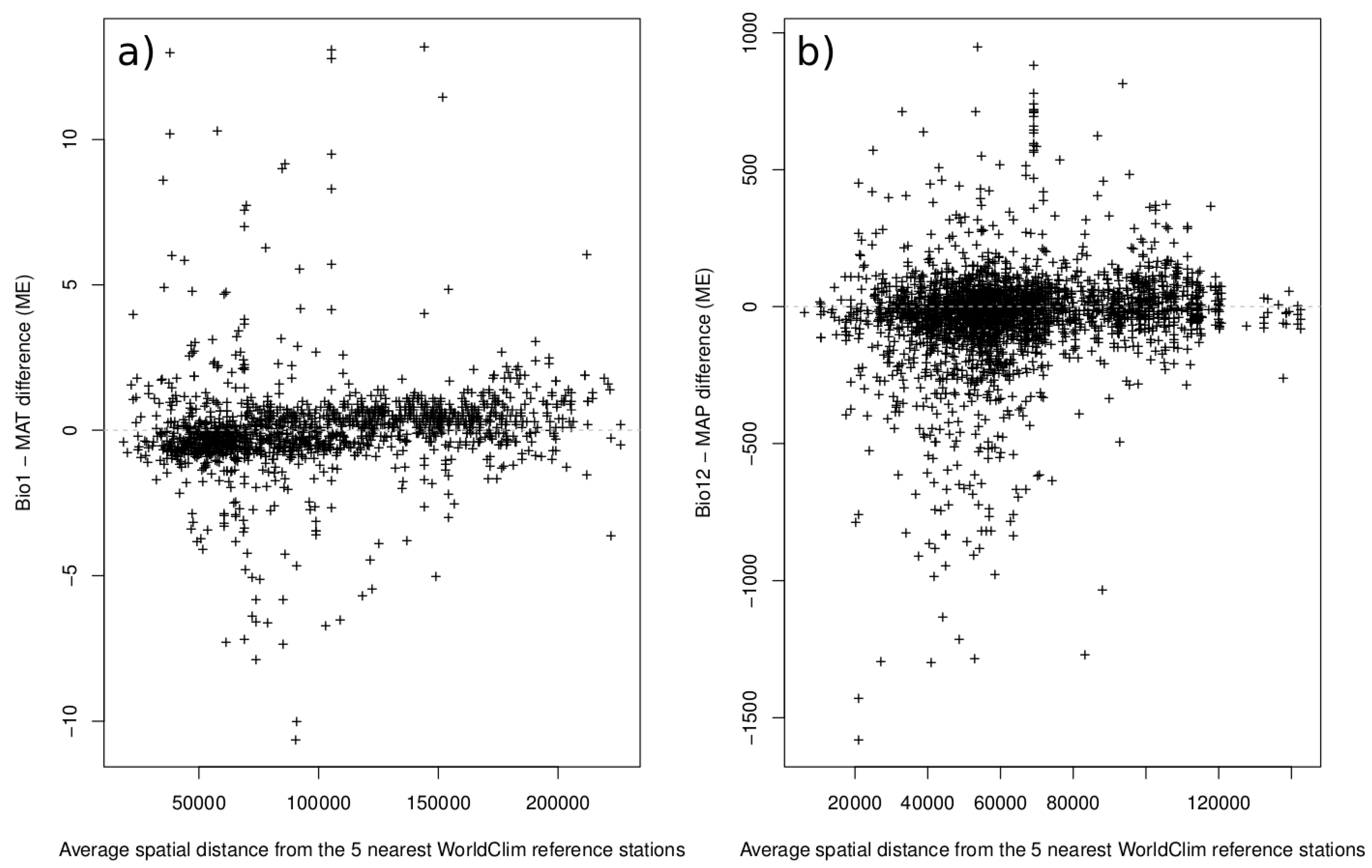
The BIO1 (mean annual air temperature) and BIO12 (mean total annual precipitation) variables of WorldClim were used as proxies to evaluate the spatial accuracy of raster surfaces. The strata were first downloaded from the official WorldClim web portal. Then, using an overlay function, the corresponding values of the two climate variables were extracted for each meteorological station in our database. A linear regression analysis was then applied to analyze the relationships between the predicted WorldClim value and the observed value in our dataset. The adjusted R2 was used to measure the amount of environmental variability expressed by WorldClim. Then the difference between the WorldClim value and the observed value (30-years normal value from our database) was calculated for each location of our database. To avoid confusion and mathematical balancing between positive and negative values, which might seriously affect the analysis, both the raw discrepancy (BIAS) and its absolute value (ABIAS) were calculated. To study possible trends across the data, we looked at the relationships between BIAS and the predictors used by the authors of WorldClim during the spatial interpolation process (i.e., latitude, longitude, elevation). Then, we retrieved the complete database of meteorological stations used by the WorldClim authors from www.arcgis.com/home/item.html?id=7644c6e78c1644b4bde2edfc44787520) and clipped to the European environment (Table 2).
We calculated the average distance of each meteorological station in our database from the geographically closest five stations in the WorldClim dataset. We expected a smaller difference where WorldClim stations were denser. Finally, the spatial autocorrelation of BIAS was evaluated using geostatistical analysis implemented in R using the gstat package [44] and modelling the semivariance of BIAS as a function of the spatial distance between records.
The whole structure of the data collection and analysis procedure is graphically reported on Figure 2.

3. Results

The compiled database included 25 European countries, albeit with an unbalanced distribution. Overall, an average of 266 records per country (both MAT and MAP) was included in the database. However, the difference among countries was huge, with a standard deviation of ± 988.64 records per country. This large standard deviation was caused by the disproportionate number of records for Sweden and Germany. Temperature (MAT) values ranged from −5.8 °C to 21.2 °C, while precipitation (MAP) was between 104.8 mm and 3318 mm. The mean difference between the interpolated WorldClim values and the observed values was 0.22 °C for temperature and −48.7mm for precipitation (Table 3), with a high coefficient of variation (6.82 for MAT and 3.40 for MAP). BIAS ranged between −10.6 °C and 13.2 °C for MAT and between −1578.1 mm and 950.8 mm for MAP. Mean ABIAS was 0.76 for MAT and 98.56 for MAP.
Results of the regression analysis for MAT and MAP are shown in Figure 3. Residuals of linear models were randomly distributed for both of the analyzed variables and were highly significant (p < 2.2 × 10⁻¹⁶). Concerning MAT, the good correlation and adequate proportion of explained variance point to a low discrepancy between the two datasets; WorldClim explained 86% of the variance (adjusted R2 = 0.856) with a residual random standard error of 1.50°C, intercept of −0.202 °C and slope almost equal to 1 (0.996). The regression line and the expected regression line for a perfect match between the two datasets almost overlapped. For MAP, 64% (adjusted R2 = 0.642) of the variance of the precipitation dataset was explained by a linear regression model, with a residual standard error of 159.6 mm. The match between the two regression lines was considerably low (Figure 3, right) with the slope of the regression coefficient higher than 1. WorldClim was characterized by higher values than observed under 500 mm precipitation and lower values above this threshold. As overall, a general overestimation of MAP values was detected in dry areas (<500 mm) with an underestimation in the remaining zones.
No relationship was found between the modelling error (ER) detected for MAT and MAP and the environmental predictors used for spatial interpolation across Europe. Modelled linear regressions explained less than 5% of variation, with one exception (Table 4). This lack of correlation can also be observed in Figure 4 where ABIAS is plotted against the average spatial distance of the “observed” meteorological station from the five WorldClim stations.
The spatial distribution of BIAS in the two most represented countries is shown in Figure 5 for the two investigated variables. Spatial aggregation is especially evident in Sweden, where most of the “large dots” are clustered in the south of the country. For Sweden and Germany, variograms of the MAP variable were fitted by means of an exponential variogram model and revealed a clear spatial autocorrelation, especially for Germany (Figure 6).

4. Discussion

The quality of the reference baseline climate has a fundamental role in predictions of the potential impact of climate change on organisms and natural ecosystems. The stability and reliability of the estimated projections calculated from species distribution models [14,45,46], management simulators [18,47], or the estimation of the geographical shift of climate zones [48] rely on the differences between current and future climate. While the representativeness of WorldClim is adequate concerning air temperatures, large differences were found in the precipitation surfaces. Our results demonstrate a systematic difference of 0.76 °C between observed and interpolated values. According to the most recent IPCC report [49], the observed increase in temperature has been around 0.2 °C per decade. As a consequence such difference might affect future projections of WorldClim dataset adding uncertainties on the further modelling efforts [22,50]. In this case a likelihood analysis should be more adequate than deterministic ones and in order to include a sensitivity analysis and evaluate the probability of success of empirical models based on phenotypic plasticity and applied future projections [51]. Precipitation, by contrast, proved to be the main weakness of WorldClim surfaces in Europe. Despite its relatively small spatial extent, the European environment is characterized by many different forest systems that reflect broad climate variability, spanning from the Mediterranean to the Arctic.
The 1961–1990 baseline period is a fundamental dataset for ecological modelling because records from earlier periods were often affected by different instrumentation or changes in observational practice [30,37]. Therefore, numerous studies from climatology to biology, ecology and forestry [36,48,52] have used this baseline period, and WorldClim has been used extensively. We can expect a further warming trend in the next two decades at a rate of about 0.1 °C per decade, due mainly to the slow response of the oceans. As a consequence, even though the linear regression analysis showed a good match between observed and interpolated data (adjusted R2 = 0.856), the difference is higher than the expected rate of change, which could heavily affect model predictions, adding uncertainties on future projections and smoothing results (i.e., land suitability projections) in an uncontrolled way [14,53,54,55]. This issue is then amplified when analysing MAP, where higher differences were found in combination with a poor regression analysis result. As a consequence, important biases may be introduced when using WorldClim’s precipitation dataset. This is particularly true when WorldClim is used as the reference line and climate projections are locally downscaled and added to the WorldClim surfaces, as in the “Delta method” [56]. As a result, the calculation of climate indices might be difficult. For example, many studies used reference evapotranspiration [57,58,59] as the main predictor in statistical models [3,60,61]. In this case, the mathematical combination of differences in MAT and MAP might introduce uncontrolled biases through the study area. These biases could represent a critical issue, especially in the Mediterranean and anywhere else that moisture deficit is identified as the most relevant climate driver.
The main advantage of our compiled dataset might be its representativeness at small scale. The authors of WorldClim themselves warn that the high resolution of the climate surfaces does not imply high data quality in all places as this depends on local climate variability, quality and density of observations and the degree of the fitted spline [31]. In a similar study, when compared with PRISM and Daymet datasets for the continental United States, many concerns were expressed, especially regarding the quality of WorldClim’s precipitation grids in mountainous areas [34,35,62,63]. For this reason, several studies at regional or national scale at higher resolution (e.g., 100–250 m) preferred the use of meteorological variables obtained at nearby observational sites [28,64,65,66]. Regardless of the distances of the investigation sites from the locations where meteorological datasets were gathered, orography and land use, and the surrounding area and variable characteristics, must be considered. At small scale their variability may be a strong driver of frequently overlooked heterogeneities, leading to significant discrepancies in transferred datasets used for otherwise appropriate processing methods [67,68].
The lack of any relationship between BIAS and the main physiographic parameters (i.e., latitude, longitude, and elevation) does not allow for any statistical adjustment (e.g., downscaling, locally calibrated lapse rate, etc.) for either temperature or precipitation. However precipitation regimes are very difficult for meteorological stations to record properly and this issue has often been found in other databases [59,69]. Many more data are required, especially in the case of forest monitoring, as a result of the lack of temporal autocorrelation during the timeframe [70].
The need for a freely available and representative global climate dataset is large and growing, as evidenced by WorldClim’s citation statistics. These goals can be achieved with local up-to-date monitoring networks, which could play a key role in evaluating global grids at small scale [71] as well as providing data for the construction of additional global climate datasets. Harmonization efforts, as well as increased representativeness of the established networks, are paramount for construction of more accurate climate surfaces. Enhanced data recovery with regular spatial coverage may overcome the lack of dense environmental or climatological sampling [28,70,72,73]. Derived surfaces are fundamental in order to plan future management strategies. For instance, and concerning forestry, additional strata, such as homogeneous climate zones, are needed as a fundamental tool to plan the transfer of genetic resources and reproductive materials across specific geographic areas [74,75]. WorldClim grids were interpolated with spline functions, a fast method known to yield results similar to polynomial functions but without mathematical instability. Such methods do not consider the spatial autocorrelation between observations, only partially achieved by more complex models where latitude and longitude are included as predictive variables [28,76]. Therefore, the exhibited spatial aggregation of the BIAS in the case of denser observations of our dataset (i.e., Sweden and Germany) may be relevant for research activities and improvements of the climate surfaces.

5. Conclusions

A new updated beta version of WorldClim has recently been released for the 1971–2000 time period. This “Version 2” (http://worldclim.org/version2), along with the need for carefully evaluating the quality of records used for modelling and keeping climate databases up-to-date, is an essential requirement for the adequate development of tools and informative systems. The lack of reliability on MAP values can be seen as the main shortcoming of the WorldClim database in Europe and elsewhere. However, precipitation is much more difficult to interpolate, given its low spatial and temporal autocorrelation as well as the lack of statistical relationships with some of the main physiographic parameters, such as elevation. Further research should focus on this parameter, seeking more significant determinants of MAP, given its importance in climate change scenarios where drought stresses are predicted to be the most relevant issue.

Author Contributions

Conceptualization, M.W., M.B. and M.M.; methodology, M.M. and M.W.; software, M.M.; validation, M.M., I.S. and M.W.; formal analysis, M.M.; investigation, M.M., M.B. and M.W.; resources, M.B.; data curation, M.M., I.S. and M.W.; writing—original draft preparation, M.M. and M.W.; writing—review and editing, M.M., I.S., M.B. and M.W.; visualization, M.M.; supervision, M.B. and M.W.; project administration, M.W. and M.B.; funding acquisition, M.M., M.W. and M.B.

Funding

Maurizio Marchi was funded by EU, in the framework of the Horizon 2020 B4EST project “Adaptive BREEDING for productive, sustainable and resilient FORESTs under climate change”, UE Grant Agreement 773383 (http://b4est.eu/). Marjana Westergren and Iztok Sinjur were funded by the Slovenian Research Agency, Research programme Forest Biology, Ecology and Technology P4-0107.

Acknowledgments

We thank Gregor Vertačnik from National Meteorological Service of Slovenia and Athanasios D. Sarantopoulos from the Hellenic National Meteorological Service Division of Climatology for contributing data.

Conflicts of Interest

The authors declare no conflict of interest.

References

  1. Fridman, J.; Holm, S.; Nilsson, M.; Nilsson, P.; Ringvall, A.H.; Ståhl, G. Adapting national forest inventories to changing requirements—The case of the Swedish national forest inventory at the turn of the 20th century. Silva Fenn. 2014, 48, 1095. [Google Scholar] [CrossRef]
  2. Bussotti, F.; Pollastrini, M. Traditional and novel indicators of climate change impacts on european forest trees. Forests 2017, 8, 137. [Google Scholar] [CrossRef]
  3. Ray, D.; Petr, M.; Mullett, M.; Bathgate, S.; Marchi, M.; Beauchamp, K. A simulation-based approach to assess forest policy options under biotic and abiotic climate change impacts: A case study on Scotland’s National Forest Estate. For. Policy Econ. 2019, 103, 17–27. [Google Scholar] [CrossRef]
  4. Marchi, M.; Ferrara, C.; Biasi, R.; Salvia, R.; Salvati, L. Agro-forest management and soil degradation in mediterranean environments: towards a strategy for sustainable land use in vineyard and olive cropland. Sustainability 2018, 10, 2565. [Google Scholar] [CrossRef]
  5. Mouchet, M.A.; Paracchini, M.L.; Schulp, C.J.E.; Stürck, J.; Verkerk, P.J.; Verburg, P.H.; Lavorel, S. Bundles of ecosystem (dis)services and multifunctionality across European landscapes. Ecol. Indic. 2017, 73, 23–28. [Google Scholar] [CrossRef] [Green Version]
  6. Dyderski, M.K.; Paź, S.; Frelich, L.E.; Jagodziński, A.M. How much does climate change threaten European forest tree species distributions? Glob. Chang. Biol. 2018, 24, 1150–1163. [Google Scholar] [CrossRef] [PubMed]
  7. Lindner, M.; Maroschek, M.; Netherer, S.; Kremer, A.; Barbati, A.; Garcia-Gonzalo, J.; Seidl, R.; Delzon, S.; Corona, P.; Kolström, M.; et al. Climate change impacts, adaptive capacity, and vulnerability of European forest ecosystems. For. Ecol. Manag. 2010, 259, 698–709. [Google Scholar] [CrossRef]
  8. Littell, J.S.; McKenzie, D.; Kerns, B.K.; Cushman, S.; Shaw, C.G. Managing uncertainty in climate-driven ecological models to inform adaptation to climate change. Ecosphere 2011, 2, art102. [Google Scholar] [CrossRef]
  9. Morton, J.F. The impact of climate change on smallholder and subsistence agriculture. Proc. Natl. Acad. Sci. USA 2007, 104, 19680–19685. [Google Scholar] [CrossRef] [Green Version]
  10. Marchetti, M.; Vizzarri, M.; Lasserre, B.; Sallustio, L.; Tavone, A. Natural capital and bioeconomy: Challenges and opportunities for forestry. Ann. Silvic. Res. 2014, 38, 62–73. [Google Scholar]
  11. Imeson, A. Desertification, Land Degradation and Sustainability; John Wiley & Sons, Inc.: New York, NY, USA, 2012; ISBN 9781119977759. [Google Scholar]
  12. Ferrarini, A.; Selvaggi, A.; Abeli, T.; Alatalo, J.M.; Orsenigo, S.; Gentili, R.; Rossi, G. Planning for assisted colonization of plants in a warming world. Sci. Rep. 2016, 6, 28542. [Google Scholar] [CrossRef] [Green Version]
  13. Chakraborty, D.; Wang, T.; Andre, K.; Konnert, M.; Lexer, M.J.; Matulla, C.; Schueler, S. Selecting populations for non-analogous climate conditions using universal response functions: The case of douglas-fir in central Europe. PLoS ONE 2015, 10, e0136357. [Google Scholar] [CrossRef]
  14. Marchi, M.; Ducci, F. Some refinements on species distribution models using tree-level national forest inventories for supporting forest management and marginal forest population detection. iForest Biogeosci. For. 2018, 11, 291–299. [Google Scholar] [CrossRef]
  15. Millar, C.I.; Stephenson, N.L.; Stephens, S.L. Climate change and forests of the future: Managing in the face of uncertainty. Ecol. Appl. 2007, 17, 2145–2151. [Google Scholar] [CrossRef]
  16. Fady, B.; Aravanopoulos, F.A.; Alizoti, P.; Mátyás, C.; von Wühlisch, G.; Westergren, M.; Belletti, P.; Cvjetkovic, B.; Ducci, F.; Huber, G.; et al. Evolution-based approach needed for the conservation and silviculture of peripheral forest tree populations. For. Ecol. Manag. 2016, 375, 66–75. [Google Scholar] [CrossRef] [Green Version]
  17. Zhang, Q.; Wei, H.; Zhao, Z.; Liu, J.; Ran, Q.; Yu, J.; Gu, W.; Zhang, Q.; Wei, H.; Zhao, Z.; et al. Optimization of the fuzzy matter element method for predicting species suitability distribution based on environmental data. Sustainability 2018, 10, 3444. [Google Scholar] [CrossRef]
  18. Castaldi, C.; Vacchiano, G.; Marchi, M.; Corona, P. Projecting nonnative Douglas fir plantations in southern europe with the forest vegetation simulator. For. Sci. 2017, 63, 101–110. [Google Scholar] [CrossRef]
  19. Subedi, N.; Sharma, M. Climate-diameter growth relationships of black spruce and jack pine trees in boreal Ontario, Canada. Glob. Chang. Biol. 2013, 19, 505–516. [Google Scholar] [CrossRef]
  20. Garzón, M.B.; Robson, T.M.; Hampe, A. ΔTraitSDM: Species distribution models that account for local adaptation and phenotypic plasticity. New Phytol. 2019, 222, 1757–1765. [Google Scholar] [CrossRef] [PubMed]
  21. Valladares, F.; Matesanz, S.; Guilhaumon, F.; Araújo, M.B.; Balaguer, L.; Benito-Garzón, M.; Cornwell, W.; Gianoli, E.; van Kleunen, M.; Naya, D.E.; et al. The effects of phenotypic plasticity and local adaptation on forecasts of species range shifts under climate change. Ecol. Lett. 2014, 17, 1351–1364. [Google Scholar] [CrossRef] [PubMed] [Green Version]
  22. O’Neill, G.A.; Hamann, A.; Wang, T.L. Accounting for population variation improves estimates of the impact of climate change on species’ growth and distribution. J. Appl. Ecol. 2008, 45, 1040–1049. [Google Scholar] [CrossRef]
  23. Noce, S.; Collalti, A.; Valentini, R.; Santini, M. Hot spot maps of forest presence in the Mediterranean basin. iForest Biogeosci. For. 2016, 9, 766–774. [Google Scholar] [CrossRef]
  24. Goberville, E.; Beaugrand, G.; Hautekèete, N.C.; Piquot, Y.; Luczak, C. Uncertainties in the projection of species distributions related to general circulation models. Ecol. Evol. 2015, 5, 1100–1116. [Google Scholar] [CrossRef] [PubMed]
  25. Noce, S.; Collalti, A.; Santini, M. Likelihood of changes in forest species suitability, distribution, and diversity under future climate: The case of Southern Europe. Ecol. Evol. 2017, 7, 9358–9375. [Google Scholar] [CrossRef] [PubMed]
  26. Pecchi, M.; Marchi, M.; Giannetti, F.; Bernetti, I.; Bindi, M.; Moriondo, M.; Maselli, F.; Fibbi, L.; Corona, P.; Travaglini, D.; et al. Reviewing climatic traits for the main forest tree species in Italy. iForest Biogeosci. For. 2019, 12, 173–180. [Google Scholar] [CrossRef] [Green Version]
  27. Attorre, F.; Alfo, M.; De Sanctis, M.; Bruno, F. Comparison of interpolation methods for mapping climatic and bioclimatic variables at regional scale. Int. J. Climatol. 2007, 1843, 1825–1843. [Google Scholar] [CrossRef]
  28. Marchi, M.; Chiavetta, U.; Castaldi, C.; Ducci, F. Does complex always mean powerful? A comparison of eight methods for interpolation of climatic data in Mediterranean area. Ital. J. Agrometeorol. 2017, 1, 59–72. [Google Scholar]
  29. Azupura, M.; Dos Ramos, K. A comparison of spatial interpolation methods for estimation of average electromagnetic field magnitude. Prog. Electromagn. Res. M 2010, 14, 135–145. [Google Scholar] [CrossRef]
  30. Mbogga, M.S.; Hamann, A.; Wang, T. Historical and projected climate data for natural resource management in western Canada. Agric. For. Meteorol. 2009, 149, 881–890. [Google Scholar] [CrossRef]
  31. Hijmans, R.J.; Cameron, S.E.; Parra, J.L.; Jones, G.; Jarvis, A. Very high resolution interpolated climate surfaces for global land areas. Int. J. Climatol. 2005, 25, 1965–1978. [Google Scholar] [CrossRef]
  32. Molyneux, N.; Soares, I.; Neto, F. Modeling current and future climates using worldclim and diva software: case studies from Timor Leste and India. J. Crop Improv. 2014, 28, 619–640. [Google Scholar] [CrossRef]
  33. Vacchiano, G.; Motta, R. An improved species distribution model for Scots pine and downy oak under future climate change in the NW Italian Alps. Ann. For. Sci. 2015, 72, 321–334. [Google Scholar] [CrossRef]
  34. Schueler, S.; Falk, W.; Koskela, J.; Lefèvre, F.; Bozzano, M.; Hubert, J.; Kraigher, H.; Longauer, R.; Olrik, D.C. Vulnerability of dynamic genetic conservation units of forest trees in Europe to climate change. Glob. Chang. Biol. 2014, 20, 1498–1511. [Google Scholar] [CrossRef]
  35. Metzger, M.J.; Bunce, R.G.H.; Jongman, R.H.G.; Sayre, R.; Trabucco, A.; Zomer, R. A high-resolution bioclimate map of the world: A unifying framework for global biodiversity research and monitoring. Glob. Ecol. Biogeogr. 2013, 22, 630–638. [Google Scholar] [CrossRef]
  36. Isaac-Renton, M.G.; Roberts, D.R.; Hamann, A.; Spiecker, H. Douglas-fir plantations in Europe: A retrospective test of assisted migration to address climate change. Glob. Chang. Biol. 2014, 20, 2607–2617. [Google Scholar] [CrossRef] [PubMed]
  37. Wang, T.; Campbell, E.M.; O’Neill, G.A.; Aitken, S.N. Projecting future distributions of ecosystem climate niches: Uncertainties and management applications. For. Ecol. Manag. 2012, 279, 128–140. [Google Scholar] [CrossRef]
  38. The R Development Core Team. R: A Language and Environment for Statistical Computing; R Foundation for Statistical Computing: Vienna, Austria, 2019. [Google Scholar]
  39. KNMI Climate Explorer. Available online: https://climexp.knmi.nl (accessed on 21 April 2016).
  40. Deutscher Wetterdienst. Available online: ftp://ftp-cdc.dwd.de/pub/CDC/observations_germany/climate/multi_annual/ (accessed on 13 April 2016).
  41. Hellenic National Meteorological Service. Available online: http://www.emy.gr/emy/en/ (accessed on 21 April 2016).
  42. National Meteorological Service of Slovenia. Available online: https://meteo.arso.gov.si/met/en/ (accessed on 21 April 2016).
  43. Swedish Meteorological and Hydrological Institute. Available online: http://www.smhi.se/klimatdata/meteorologi/temperatur/dataserier-med-normalvarden-1.7354 (accessed on 30 March 2016).
  44. Pebesma, E.J. Multivariable geostatistics in S: The gstat package. Comput. Geosci. 2004, 30, 683–691. [Google Scholar] [CrossRef]
  45. Zhang, L.; Liu, S.; Sun, P.; Wang, T.; Wang, G.; Zhang, X.; Wang, L. Consensus forecasting of species distributions: the effects of niche model performance and niche properties. PLoS ONE 2015, 10, e0120056. [Google Scholar] [CrossRef]
  46. Hamann, A.; Roberts, D.R.; Barber, Q.E.; Carroll, C.; Nielsen, S.E. Velocity of climate change algorithms for guiding conservation and management. Glob. Chang. Biol. 2015, 21, 997–1004. [Google Scholar] [CrossRef]
  47. Mairota, P.; Leronni, V.; Xi, W.; Mladenoff, D.J.; Nagendra, H. Using spatial simulations of habitat modification for adaptive management of protected areas: Mediterranean grassland modification by woody plant encroachment. Environ. Conserv. 2013, 41, 144–156. [Google Scholar] [CrossRef]
  48. Belda, M.; Holtanová, E.; Kalvová, J.; Halenka, T. Global warming-induced changes in climate zones based on CMIP5 projections. Clim. Res. 2016, 71, 17–31. [Google Scholar] [CrossRef] [Green Version]
  49. IPCC. Climate Change 2014: Impacts, Adaptation, and Vulnerability. Part A: Global and Sectoral Aspects. Contribution of Working Group II to the Fifth Assessment Report of the Intergovernmental Panel on Climate Change; Field, C.B., Barros, V.R., Dokken, D.J., Eds.; Cambridge University Press: Cambridge, UK; New York, NY, USA, 2014; p. 1132. [Google Scholar]
  50. Wood, S.N. On confidence intervals for generalized additive models based on penalized regression splines. Aust. N. Z. J. Stat. 2006, 48, 445–464. [Google Scholar] [CrossRef]
  51. Fréjaville, T.; Fady, B.; Kremer, A.; Ducousso, A.; Garzón, M.B. Inferring phenotypic plasticity and local adaptation to climate across tree species ranges using forest inventory data. bioRxiv 2019, 1–34. [Google Scholar] [CrossRef]
  52. Ray, D.; Bathgate, S.; Moseley, D.; Taylor, P.; Nicoll, B.; Pizzirani, S.; Gardiner, B. Comparing the provision of ecosystem services in plantation forests under alternative climate change adaptation management options in Wales. Reg. Environ. Chang. 2015, 15, 1501–1513. [Google Scholar] [CrossRef]
  53. Bellucci, A.; Gualdi, S.; Masina, S.; Storto, A.; Scoccimarro, E.; Cagnazzo, C.; Fogli, P.; Manzini, E.; Navarra, A. Decadal climate predictions with a coupled OAGCM initialized with oceanic reanalyses. Clim. Dyn. 2013, 40, 1483–1497. [Google Scholar] [CrossRef]
  54. Heikkinen, R.K.; Luoto, M.; Araújo, M.B.; Virkkala, R.; Thuiller, W.; Sykes, M.T. Methods and uncertainties in bioclimatic envelope modelling under climate change. Prog. Phys. Geogr. 2006, 30, 751–777. [Google Scholar] [CrossRef] [Green Version]
  55. Perdinan, P.; Winkler, J.A. Changing human landscapes under a changing climate: Considerations for climate assessments. Environ. Manag. 2014, 53, 42–54. [Google Scholar] [CrossRef]
  56. Ramirez-Villegas, J.; Jarvis, A. CIAT Decision and Policy Analysis Working Paper; CIAT: London, UK, 2010; p. 18. [Google Scholar]
  57. Hargreaves, G.H.; Samani, Z.A. Reference crop evapotranspiration from temperature. Appl. Eng. Agric. 1985, 1, 96–99. [Google Scholar] [CrossRef]
  58. Maca, P.; Pech, P. Forecasting SPEI and SPI drought indices using the integrated artificial neural networks. Comput. Intell. Neurosci. 2016, 2016, 3868519. [Google Scholar] [CrossRef]
  59. Vicente-Serrano, S.M.; Beguería, S.; López-Moreno, J.I.; Angulo, M.; El Kenawy, A. A new global 0.5° gridded dataset (1901–2006) of a multiscalar drought index: Comparison with current drought index datasets based on the palmer drought severity index. J. Hydrometeorol. 2010, 11, 1033–1043. [Google Scholar] [CrossRef]
  60. Svenning, J.C.; Fitzpatrick, M.C.; Normand, S.; Graham, C.H.; Pearman, P.B.; Iverson, L.R.; Skov, F. Geography, topography, and history affect realized-to-potential tree species richness patterns in Europe. Ecography (Cop.) 2010, 33, 1070–1080. [Google Scholar] [CrossRef]
  61. Colantoni, A.; Ferrara, C.; Perini, L.; Salvati, L. Assessing trends in climate aridity and vulnerability to soil degradation in Italy. Ecol. Indic. 2015, 48, 599–604. [Google Scholar] [CrossRef]
  62. Hannachi, A.; Jolliffe, I.T.; Stephenson, D.B. Empirical orthogonal functions and related techniques in atmospheric science: A review. Int. J. Climatol. 2007, 27, 1119–1152. [Google Scholar] [CrossRef]
  63. Daly, C.; Halbleib, M.; Smith, J.I.; Gibson, W.P.; Doggett, M.K.; Taylor, G.H.; Curtis, J.; Pasteris, P.P. Physiographically sensitive mapping of climatological temperature and precipitation across the conterminous United States. Int. J. Climatol. 2008, 28, 2031–2064. [Google Scholar] [CrossRef]
  64. Blasi, C.; Chirici, G.; Corona, P.; Marchetti, M.; Maselli, F.; Puletti, N. Spazializzazione di dati climatici a livello nazionale tramite modelli regressivi localizzati. Forest 2007, 4, 213–219. [Google Scholar] [CrossRef]
  65. Wang, T.; Hamann, A.; Spittlehouse, D.; Carroll, C. Locally downscaled and spatially customizable climate data for historical and future periods for North America. PLoS ONE 2016, 11, e0156720. [Google Scholar] [CrossRef]
  66. Harris, I.; Jones, P.D.; Osborn, T.J.; Lister, D.H. Updated high-resolution grids of monthly climatic observations—The CRU TS3.10 Dataset. Int. J. Climatol. 2014, 34, 623–642. [Google Scholar] [CrossRef]
  67. Falk, W.; Mellert, K.H. Species distribution models as a tool for forest management planning under climate change: Risk evaluation of Abies Alba in Bavaria. J. Veg. Sci. 2011, 22, 621–634. [Google Scholar] [CrossRef]
  68. Trivedi, M.R.; Berry, P.M.; Morecroft, M.D.; Dawson, T.P. Spatial scale affects bioclimate model projections of climate change impacts on mountain plants. Glob. Chang. Biol. 2008, 14, 1089–1103. [Google Scholar] [CrossRef] [Green Version]
  69. Marchi, M.; Castaldi, C.; Merlini, P.; Nocentini, S.; Ducci, F. Stand structure and influence of climate on growth trends of a Marginal forest population of Pinus nigra spp. nigra. Ann. Silvic. Res. 2015, 39, 100–110. [Google Scholar]
  70. Ferrara, C.; Marchi, M.; Fares, S.; Salvati, L. Sampling strategies for high quality time-series of climatic variables in forest resource assessment. iForest Biogeosci. For. 2017, 10, 739–745. [Google Scholar] [CrossRef] [Green Version]
  71. Way, R.G.; Oliva, F.; Viau, A.E. Underestimated warming of northern Canada in the Berkeley Earth temperature product. Int. J. Climatol. 2017, 37, 1746–1757. [Google Scholar] [CrossRef]
  72. Bhowmik, A.K.; Costa, A.C. Representativeness impacts on accuracy and precision of climate spatial interpolation in data-scarce regions. Meteorol. Appl. 2014, 22, 368–377. [Google Scholar] [CrossRef]
  73. Wong, D.W.; Yuan, L.; Perlin, S. A comparison of spatial interpolation methods for the estimation of air quality data. J. Expo. Anal. Environ. Epidemiol. 2004, 14, 404–415. [Google Scholar] [CrossRef] [PubMed]
  74. Metzger, M.J.; Brus, D.J.; Bunce, R.G.H.; Carey, P.D.; Gonçalves, J.; Honrado, J.P.; Jongman, R.H.G.; Trabucco, A.; Zomer, R. Environmental stratifications as the basis for national, European and global ecological monitoring. Ecol. Indic. 2013, 33, 26–35. [Google Scholar] [CrossRef] [Green Version]
  75. De Dato, G.; Teani, A.; Mattioni, C.; Marchi, M.; Monteverdi, M.C.; Ducci, F. Delineation of seed collection zones based on environmental and genetic characteristics for Quercus suber L. in Sardinia, Italy. iForest Biogeosci. For. 2018, 11, 651–659. [Google Scholar] [CrossRef]
  76. Bachmaier, M.; Backes, M. Variogram or Semivariogram? Variance or Semivariance? Allan Variance or Introducing a New Term? Math. Geosci. 2011, 43, 735–740. [Google Scholar] [CrossRef]
Figure 1. Spatial distribution of the compiled dataset for: (a) temperature records and (b) precipitation records. Each dot represents a meteorological station. The darker the area, the more data were retrieved.
Sustainability 11 03043 g001
Figure 2. Flowchart of the data collection and statistical analysis we made to test the reliability of WorlClim version 1 data.
Sustainability 11 03043 g002
Figure 3. Results of the regression analysis for: (a) temperature represented by Bio1 variable of WorldClim database on x-axis and (b) precipitation represented by Bio12 variable of WorldClim database versus observed values on the y-axis. Regression coefficients at top-left of each figure. The 1:1 line of a perfect match shown dashed.
Sustainability 11 03043 g003
Figure 4. Relationship between the detected differences (WorldClim value, observed) and the average spatial distance of the observed record (new database) from the five nearest WorldClim reference stations for (a) temperature and (b) precipitation.
Sustainability 11 03043 g004
Figure 5. Spatial distribution of ABIAS for temperature (a and b) and precipitation (c and d) across Sweden and Germany, the two most sampled countries in the database. The larger the gray dot, the greater the difference between WorldClim and the independent dataset.
Sustainability 11 03043 g005
Figure 6. (Semi)variograms for precipitation calculated by the gstat package in R for Sweden (a) and Germany (b). There is a rather clear spatial structure that might be used as input for further geostatistical procedures (i.e., kriging) in order to adjust WorldClim raster maps.
Sustainability 11 03043 g006
Table 1. Structure of the compiled database.
CountryTotal MeteostationsMAT RecordsMAP RecordsData Source
Albania333[39]
Austria232123
Belgium999
Bulgaria181818
Croatia111
Czech201920
Denmark444
Finland181718
France767576
Germany48257194733[40]
Greece262526[41]
Hungary999[39]
Ireland666
Italy303030
North Macedonia111
Montenegro111
Netherlands555
Norway181818
Portugal181818
Slovakia141414
Slovenia424242[42]
Spain515151[39]
Sweden13916041351[43]
Switzerland121112[39]
United Kingdom383837
TOTAL665917596526
MEAN26670261
ST. DEV988.64179.54969.08
Table 2. Number of meteorological stations per country used by Hijmans et al. [31] in Europe.
CountryTemperaturePrecipitationCountryTemperaturePrecipitation
Albania07Latvia39
Andorra00Liechtenstein00
Armenia22Lithuania1619
Austria325Luxembourg16
Belarus822North Macedonia77
Belgium318Malta13
Bosnia and Herz.710Moldova23
Bulgaria415Monaco00
Croatia1313Montenegro52
Czech Republic716Netherlands710
Denmark1941Norway854
Estonia312Poland1863
Faeroe Islands11Portugal1618
Finland1932Romania1128
France82107Russia44124
Georgia120San Marino00
Germany89116Serbia2312
Gibraltar01Slovakia310
Greece2648Slovenia62
Guernsey00Spain60117
Hungary820Sweden1660
Ireland1651Switzerland820
Isle of Man01Turkey513548
Italy133151Ukraine2281
Jersey03UK29188
Summary statisticsTemperature recordsPrecipitation records
TOTAL12632116
MEAN2542
SD74.8684.89
Table 3. Difference between local data and WorldClim’s surfaces.
VariableAVRSDCVMAXMINABSAVR
MAT [°C]0.221.506.82−10.6213.210.76
MAP [mm]−48.70165.353.40−1578.10950.8098.56
AVR = average value; SD = standard deviation; CV = coefficient of variation; MAX = maximum difference; MIN = minimum difference; ABSAVR = average of absolute values.
Table 4. Linear regression parameters when modelling error (ER) and the environmental predictors. Each predictor was tested separately (ADF5NM=Average distance from the five nearest meteorological stations).
VariablePredictorInterceptSlopeExplained Variancep-Value
MATLatitude0.290.0000000.56%0.00092
Longitude−0.340.0000001.20%0.00000
Elevation0.54−0.0010254.95%0.00000
ADF5NM0.090.0000020.18%0.04138
MAPLatitude−45.160.0000140.05%0.04492
Longitude−202.280.0000614.33%0.00000
Elevation8.15−0.20669010.26%0.00000
ADF5NM−107.020.0010591.61%0.00000

