Article

Estimation of Carbon Fluxes from Eddy Covariance Data and Satellite-Derived Vegetation Indices in a Karst Grassland (Podgorski Kras, Slovenia)

1
Slovenian Forestry Institute, 1000 Ljubljana, Slovenia
2
Biotechnical Faculty, University of Ljubljana, 1000 Ljubljana, Slovenia
3
Department of Agri-Food, Animal and Environmental Sciences, University of Udine, 33100 Udine, Italy
4
Forest Research Center, University of Lisbon, 1349-017 Lisbon, Portugal
*
Author to whom correspondence should be addressed.
Remote Sens. 2019, 11(6), 649; https://doi.org/10.3390/rs11060649
Submission received: 19 January 2019 / Revised: 12 March 2019 / Accepted: 13 March 2019 / Published: 16 March 2019
(This article belongs to the Special Issue Remote Sensing of Primary Productivity)

Abstract

:
The Eddy Covariance method (EC) is widely used for measuring carbon (C) and energy fluxes at high frequency between the atmosphere and the ecosystem, but has some methodological limitations and a spatial restriction to an area, called a footprint. Remotely sensed information is usually used in combination with eddy covariance data in order to estimate C fluxes over larger areas. In fact, spectral vegetation indices derived from available satellite data can be combined with EC measurements to estimate C fluxes outside of the tower footprint. Following this approach, the present study aimed to model C fluxes for a karst grassland in Slovenia. Three types of model were considered: (1) a linear relationship between Net Ecosystem Exchange (NEE) or Gross Primary Production (GPP) and each vegetation index; (2) a linear relationship between GPP and the product of a vegetation index with PAR (Photosynthetically Active Radiation); and (3) a simplified LUE (Light Use-Efficiency) model assuming a constant LUE. We compared the performance of several vegetation indices derived from two remote platforms (Landsat and Proba-V) as predictors of NEE and GPP, based on three accuracy metrics, the coefficient of determination (R2), the Root Mean Square Error (RMSE) and the Akaike Information Criterion (AIC). Two types of aggregation of flux data were explored: midday average and daily average fluxes. The vapor pressure deficit (VPD) was used to separate the growing season into two phases, a wet and a dry phase, which were considered separately in the modelling process, in addition to the growing season as a whole. The results showed that NDVI is the best predictor of GPP and NEE during the wet phase, whereas water-related vegetation indices, namely LSWI and MNDWI, were the best predictors during the dry phase, both for midday and daily aggregates. Model 1 (linear relationship) was found to be the best in many cases. The best regression equations obtained were used to map GPP and NEE for the whole study area. Digital maps obtained can practically contribute, in a cost-effective way to the management of karst grasslands.

Graphical Abstract

1. Introduction

Grasslands are among the most widespread vegetation types worldwide, covering between 14% and 26% of the earth’s surface [1,2]. They play an important role in the carbon (C) cycle, as they store about 23% of the global soil C [3] and, given the contribution of grasslands in mitigating climate change, it is important to monitor their C sequestration potential.
The Eddy Covariance (EC) method permits to measure, at an ecosystem scale, the atmosphere-ecosystem exchange of water, energy and CO2 fluxes [4]. It provides a reliable direct measurement of different gas compounds together with meteorological variables, at high temporal detail, making it possible to ascertain the influence of climate drivers or other disturbances/stress factors on fluxes at ecosystem scale [5]. The EC measurements represent fluxes in an area around the tower (named footprint) whose size and shape depend on the set-up of the equipment, the structure and height of the canopy and wind direction and speed. This spatial limitation raises the necessity to estimate C fluxes outside the footprint of an EC tower, since it would be costly and unfeasible to install towers to cover all areas of interest.
The net ecosystem exchange (NEE) is the balance between two components, the respiration of the ecosystem (Reco) and the gross primary production (GPP), which represents the amount of carbon fixed through photosynthesis [6,7]. A possible approach to estimate GPP outside the limits of the footprint of an EC tower is the use of remotely sensed information [8]. Light-use efficiency (LUE) models are the most frequently applied to estimate GPP from spectral vegetation indices (VIs) remotely retrieved [9].
The LUE concept states that GPP is directly related to the absorbed photosynthetically active radiation (APAR) and photosynthetic efficiency by Photosynthetically Active Radiation (PAR) unit, which can be reduced under environmental stresses such as low temperatures or water stress [10,11]. Thanks to the empirical relationship that exists between the fraction of absorbed photosynthetically-active radiation (fAPAR) and VIs [10,11,12], the latter are used in many studies as proxies of GPP. The most widely used VIs to that end are the Normalized Difference Vegetation Index (NDVI) and the Enhanced Vegetation Index (EVI), which are empirically known to be good metrics of green biomass [8,9,13,14]. NDVI is more sensitive to background reflectance and tends to saturate at high leaf area, which makes EVI a good alternative, as it is less sensitive to these limitations [14,15]. Some VIs similar to NDVI and EVI have also been used, such as the Green Normalized Difference Vegetation Index (GNDVI) which is more sensitive to chlorophyll content in plants than NDVI [16,17], and the Soil-Adjusted Vegetation Index (SAVI) which is derived from NDVI by including a soil-adjustment factor [18]. In grasslands, several greenness-related VIs demonstrated their suitability as proxies of GPP. The MERIS Terrestrial Chlorophyll Index (MTCI) was found to provide the best estimates of GPP in subalpine grasslands [19,20], EVI and SAVI were the best predictors of GPP in a temperate-alpine grassland [14], MTCI, PSRI (Plant Senescence Reflectance Index) and GNDVI revealed their suitability in a Mediterranean grassland [17]. Other studies revealed the usefulness of water-related vegetation indices. In this regard, other VIs used to depict the water content in plants such as Normalized Difference Surface Water Index (NDSWI), Land Surface Water Index (LSWI) and Modified Normalized Difference Water Index (MNDWI) [13,21,22] could also be useful, since they are more sensitive to drought than greenness-related VIs, which makes them likely the best VIs in the estimation of C fluxes in ecosystems undergoing seasonal drought [23]. In most studies, the selection of VIs [14,17,19] is limited by the availability of remote information from satellite platforms.
An important input of LUE models is the LUE term. While some studies recently attempted to estimate LUE based on some indices such as the photochemical reflectance index (PRI) or the sun induced chlorophyll fluorescence (SIF) [19,24], other studies considered the LUE term as a biome-specific constant [25], one which is usually dependent on seasonal changes [19,26]. Besides LUE models, empirical models based on the relationship observed between VIs or the product VIs *PAR and GPP were also successfully frequently applied [9,19,27,28]. In addition, since photosynthesis (GPP) and respiration (Reco) are generally positively correlated [29,30,31], reliable estimates of both NEE and GPP have been obtained from remote sensing products.
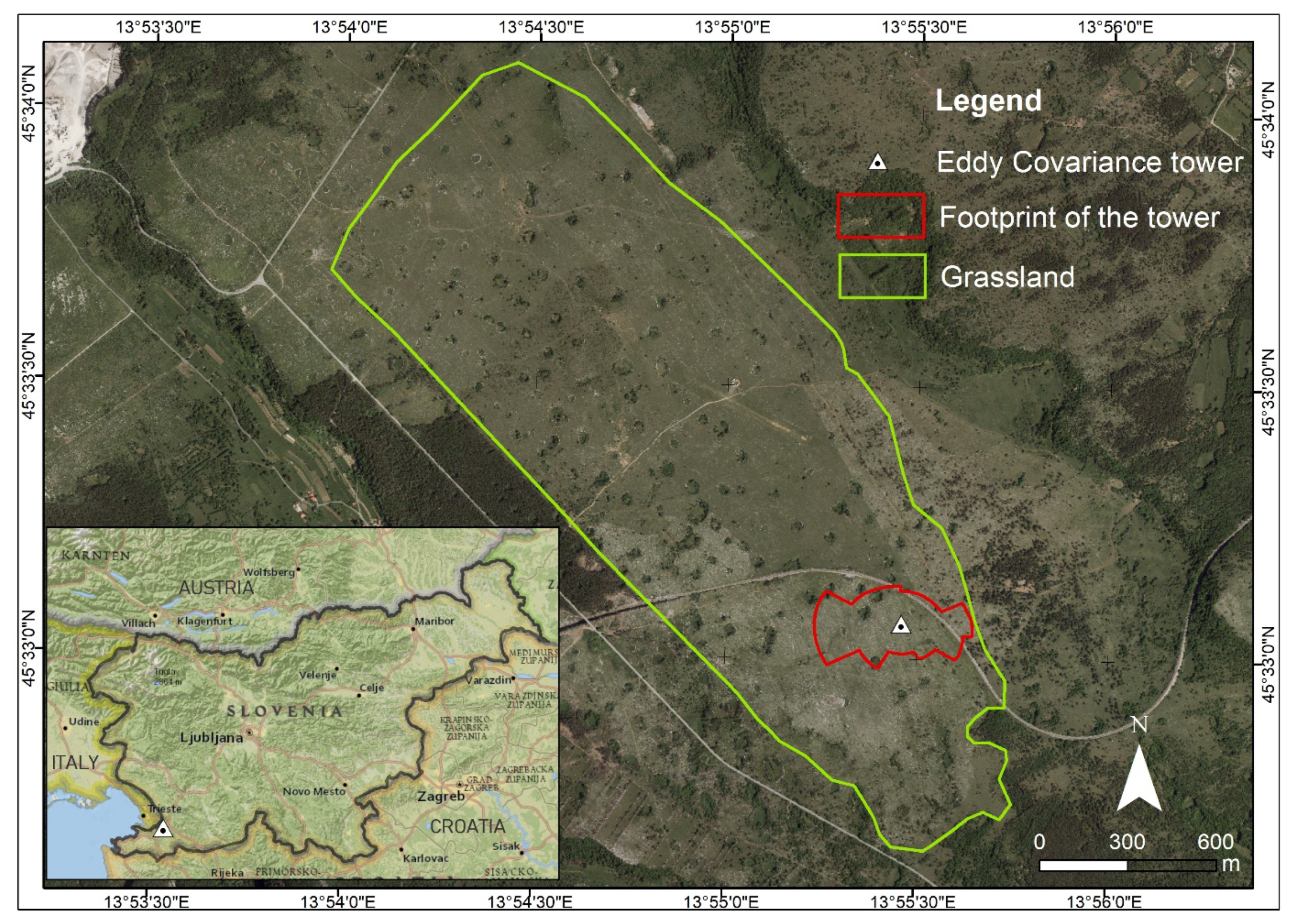
Grasslands in the Slovenian Karst represent an important resource, as they are one of the first colonizers of shallow soils found in the area. In addition, they are important biodiversity hotspots, are used as extensive pastures by local populations, and contribute to sequestering C in soils [32]. With climate change, more uncertainty could arise regarding the provision of the aforementioned ecosystem goods and services. Thus, thematic digital maps reporting GPP and NEE estimates in the region might provide short-term information on the ecosystem’s response to climate in an easy, cost-efficient way, with advantages for stakeholders engaged in grasslands productivity and sustainability.
The objective of this study was to estimate NEE and GPP for a karst grassland in the Podgorski Kras plateau (Slovenia) by combining both EC and satellite data in order to provide a basis for large-scale monitoring of the C balance in the grasslands of this region. To that end, we aimed to:
(i)
Evaluate the ability of different VIs retrieved from remote sensing platforms to represent GPP and NEE trends in a karst grassland;
(ii)
Compare the performance of different models, integrating VIs in the estimation of GPP and NEE;
(iii)
Apply obtained results to map NEE and GPP for the grassland area in the Podgorski Kras Plateau comparing the suitability of different remote platforms.

2. Materials and Methods

2.1. Study Area

The present study was conducted in the Podgorski Kras plateau located in the sub-mediterranean region of south-west Slovenia (longitude 13°55′27.714″E; latitude 45°33′2.858″N). The area has undergone major human influences due to its position at the transition between the Mediterranean and central Europe. In fact, agricultural practices such as overgrazing in the past centuries led to pronounced destruction of the vegetation cover, causing severe soil erosion and resulting into a stony and bare landscape. However, thanks to the economic development causing the near-abandonment of agriculture practices in the area, a succession is taking place and different vegetation types, ranging from grasslands to secondary oak forests, are now present [33].
The bedrock is mainly composed of limestone from Paleocene and Eocene [34]. The chemical weathering known as karst phenomena led to the formation of Leptosols and Cambisols, which represent insoluble fractions of carbonates. As a result, the soil is superficial, with depths ranging from 0 cm to several decimeters in soil pockets between rocks. The organic matter represents about 12–15% of the topsoil [33].
The climate is often referred to as sub-Mediterranean, with a mean annual temperature of 10.5 °C, a mean daily temperature of 1.8 °C and 19.9 °C in January and June respectively, and an average annual precipitation around 1370 mm. Climate statistics represent 30 years’ average (1971–2000) of four meteorological stations in the region [35]. Winters are windy (Bora wind), with periodic snow cover. The growing season ranges from March or April to October [33].
The present study considered a homogenous grassland (Figure 1), where only herbaceous species were present with the exception of few shrubs. The most abundant species were Bromopsis erecta (Huds.) Fourr., Carex humilis Leyss., Stipa eriocaulis Borb., Centaurea rupestris L., Potentilla tommasiniana F.W. Schultz, Anthyllis vulneraria L., Galium corrudifolium Vill. and Teucrium montanum L.

2.2. Data Acquisition

2.2.1. Eddy Covariance and Meteorological Data

In order to monitor CO2 and H2O fluxes between the grassland and the atmosphere, an eddy covariance tower was installed as reported in Figure 1 in 2008 [36], providing continuous measurements of NEE and water exchanges between the grassland and the atmosphere. The eddy covariance system consists of an open path infrared gas (CO2 and H2O) analyzer (LI-7500, Li-Cor, Lincoln, NE, USA) and a sonic anemometer (WindMaster 1590-PK, GILL, Hampshire, UK), installed at a height of 2 m. Flux data were recorded at 10 Hz and then averaged half-hourly, for an estimated footprint of 195 m using the model after [37]. The applied methodology for preparing the flux data was based on the Euroflux protocol [38] with the Webb Pearman Leuning correction [39] and method 4 of Burba correction [40]. All post processing elaborations and frequency response corrections have been performed using EdiRe Data software [41], and quality assessment and quality check analysis (QA/QC) were conducted according to [42]. The weather station provides measurements of environmental variables such as soil temperature and soil water content, both at a depth of 10 cm, incoming short-wave radiation (Rg), air temperature (Tair), humidity, soil heat flux and precipitation (P). All these measurements were taken at 0.1 Hz and then averaged at half-hour time step [36]. Since PAR can be estimated as a constant fraction of shortwave radiation [43], in this study, we adopted Rg values instead of PAR.
Tair and Rg data were gap-filled based on data from a nearby meteorological station in Koper (at a distance of 15 km from the tower). NEE data were partitioned into GPP and Reco according to [44] using daytime data-based estimates, considering temperature sensitivity of respiration and VPD limitation of GPP.

2.2.2. Spectral Vegetation Indices

In this study, two sources of remotely-sensed data were considered. The 300 m resolution NDVI data, consisting of 10 days aggregates of NDVI, provided by the Proba-V platform (NDVIPV) and available for the whole world since 2014 were downloaded from Copernicus global land service portal [45]. Landsat 8 operational land imager (OLI) images (30 m resolution) were downloaded from the portal of the United States Geological survey [46] for the growing season (March to October) from 2014 to 2017. Landsat 8 images have a temporal resolution of 16 days. However, cloud cover rendered most of them useless [47,48] for our study. Selected images included only available images with no or insignificant cloud cover in the footprint of the tower. Contrarily to NDVIPV data, Landsat images represent single date images. The Table 1 presents the different bands of Landsat 8 and those of Proba-V satellite.
Landsat 8 surface reflectance data are available at [49]. In this study however, we conducted the preprocessing from raw images. Once downloaded, the Landsat images underwent a radiometric calibration to convert radiance values to top of atmosphere reflectance, followed by an atmospheric correction through dark object subtraction in order to remove atmospheric components such as scattering and absorption of solar energy in the atmosphere, and to obtain top of canopy reflectance [50]. The image processing was conducted with the ENVI 5.1 software.
The corrected images were used to compute the different vegetation indices (Table 2, except NDVIPV). An average value for each index was computed for the pixels in the footprint of the tower (Figure 1) using the Raster package in R software [51].
Despite the availability of flux data since 2008, only a timeframe of four years (2014–2017) was considered in order to match the timeframe of the remote sensing information available for this study. In total, for the growing seasons and excluding periods with large gaps of eddy covariance data, the number of NDVIPV and Landsat images used in the study were 70 and 39, respectively.

2.3. Data Analysis and Modelling

The general approach consisted of flux and environmental parameters aggregation, followed by regressions between aggregated fluxes and VIs. Two types of aggregation of flux data were considered. For the first data aggregation type, midday (between 11 a.m. and 4 p.m.) averages of half-hourly fluxes were calculated as in [9]. For the second type of aggregation, we calculated daily averages of half-hourly fluxes. For further analysis, midday and daily aggregated flux data were subsequently averaged over different time steps as follows: for NDVIPV data, aggregated flux data were averaged over 10 days period to match temporal aggregation provided by Proba-V. For VIs derived from Landsat 8 images, midday and daily flux data were averaged over 5 days (acquisition date plus 4 days prior to this date), since a preliminary test showed a better correlation if aggregated fluxes were considered instead of the overpass day only.
Three types of model linking VIs and EC data were tested in this study after [19]:
  • (i) Model 1 assuming a direct linear relationship between GPP or NEE and a vegetation index
    NEE or GPP = a*VI + b,
    where NEE is the net ecosystem exchange, GPP is the gross primary production, VI is a vegetation index, a and b are regression constants.
  • (ii) Model 2 assuming a direct linear relationship between GPP and the product of a VI and incoming PAR or Rg in this study
    GPP = a*(VI*Rg) + b,
    where GPP is the gross primary production, VI is a vegetation index, Rg is the short-wave radiation, a and b are regression constants.
  • (iii) Model 3, a simplified LUE model, in which the LUE term is considered a constant (integrated in the model) and APAR is obtained by multiplying the fraction of absorbed photosynthetically active radiation (fAPAR), estimated as a linear function of a VI, by PAR (replaced by Rg in this study). By this approach, LUE and fAPAR estimates are conceptually independent.
    GPP = LUE* (a*VI + b)*Rg,
    where GPP is the gross primary production, LUE is the light use efficiency, VI is a vegetation index, Rg is the short-wave radiation, a and b are regression constants.
All three models were implemented for the entire growing season (single) or splitting the growing season in two phases (wet and dry). When stressed by low soil water content (SWC) or high vapor pressure deficit (VPD), plants close stomata, reducing transpiration and photosynthesis [10,57,58]. Therefore, SWC and VPD could be used as proxies for water stress. Based on our measurements, evapotranspiration was more sensitive to an increase in VPD than a decrease in SWC and a threshold value of 1500 Pa was considered to separate the wet phase from the dry phase of the growing season. A VPD value of 1500 Pa was also reported to be the optimal VPD for stomatal conductance in grasslands [59,60]. Above this value, plant activity would reduce progressively. We therefore defined the wet phase as the period of the growing season with midday average VPD less than or equal to 1500 Pa, and the dry phase as the period of the growing season with midday average VPD greater than 1500 Pa (June–August). The equation 3 was applied to each phase, assuming a constant LUE within the phase.
In order to compare the performance of the different vegetation indices as proxies of carbon fluxes in the different regressions, three accuracy metrics were computed, namely the coefficient of determination (R2), the Root Mean Square Error (RMSE) and the Akaike Information Criterion (AIC). Additionally, in order to validate our models, we applied a bootstrap simulation with 1000 iterations to obtain the mean coefficient of determination (R2boot) with a 95% confidence interval for each regression [61,62,63]. The best models are the ones with a high value of R2 and a low value of RMSE and AIC.
Applying the best selected models, estimates of GPP and NEE per growing season were computed based on NDVIPV data for years 2014 to 2017.
All analyses were done using the R software, version 3.4.4 [51].

2.4. Mapping of Carbon Fluxes

The selected models were then used to create illustrative GPP and NEE maps of the study area for two dates, as example of a wet and dry period. Image algebra was performed on a vegetation index layer based on the expression of each model. The maps were created using the ArcGIS 10.4.1 software. The resulting GPP and NEE represent average fluxes of 5 or 10 days, if estimated from Landsat derived VIs or NDVIPV respectively.

3. Results

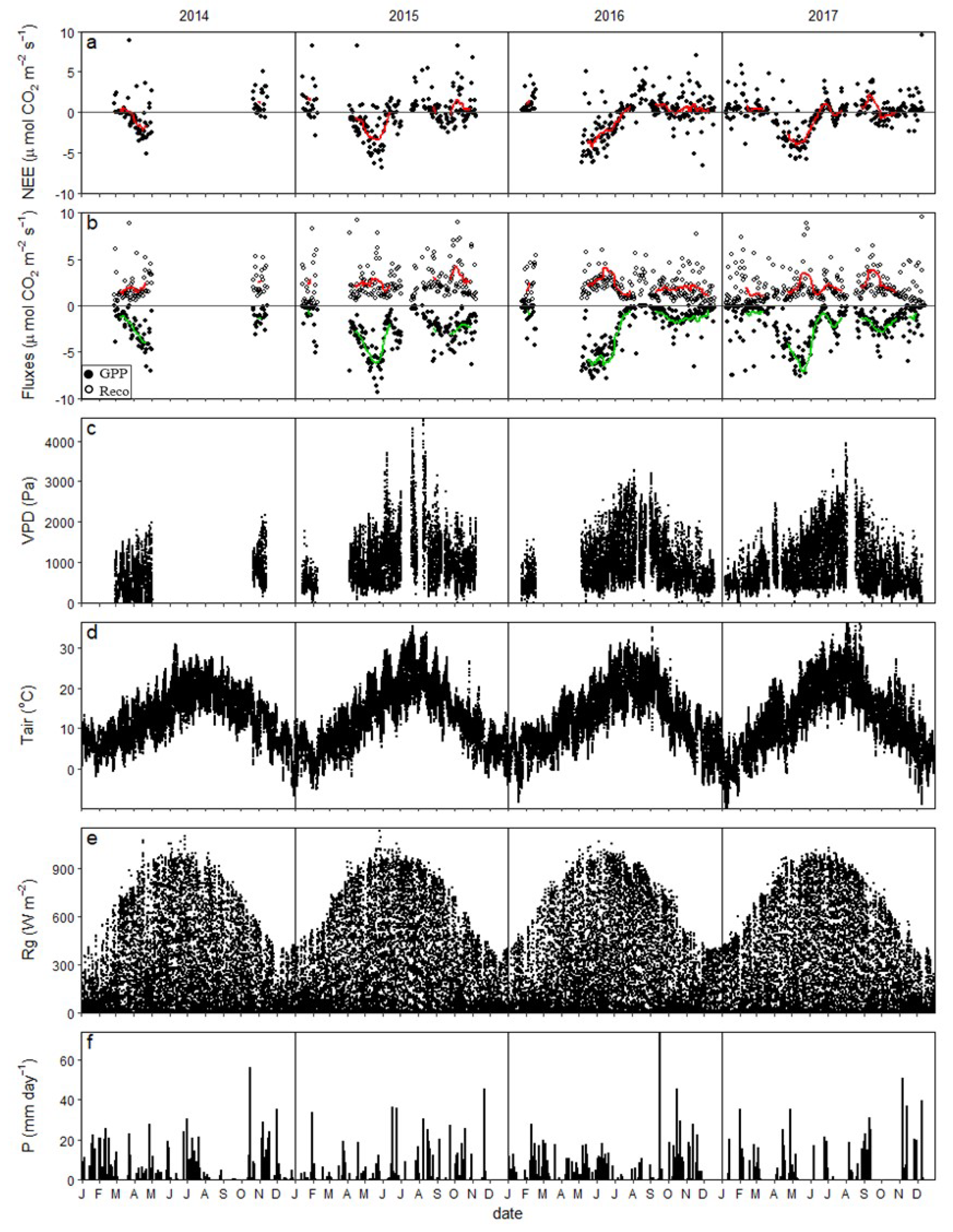
3.1. Carbon Fluxes and Environmental Variables Measured by the EC Tower

Fluxes (NEE, GPP, Reco) and main meteorological variables (VPD, Tair, Rg and P) are reported for the whole study period (2014–2017) in Figure 2. Large gaps due to power problems are noticeable for flux data. Tair and Rg show no gaps because they were gap-filled using data from a nearby meteorological station in Koper.

3.2. Vegetation Indices

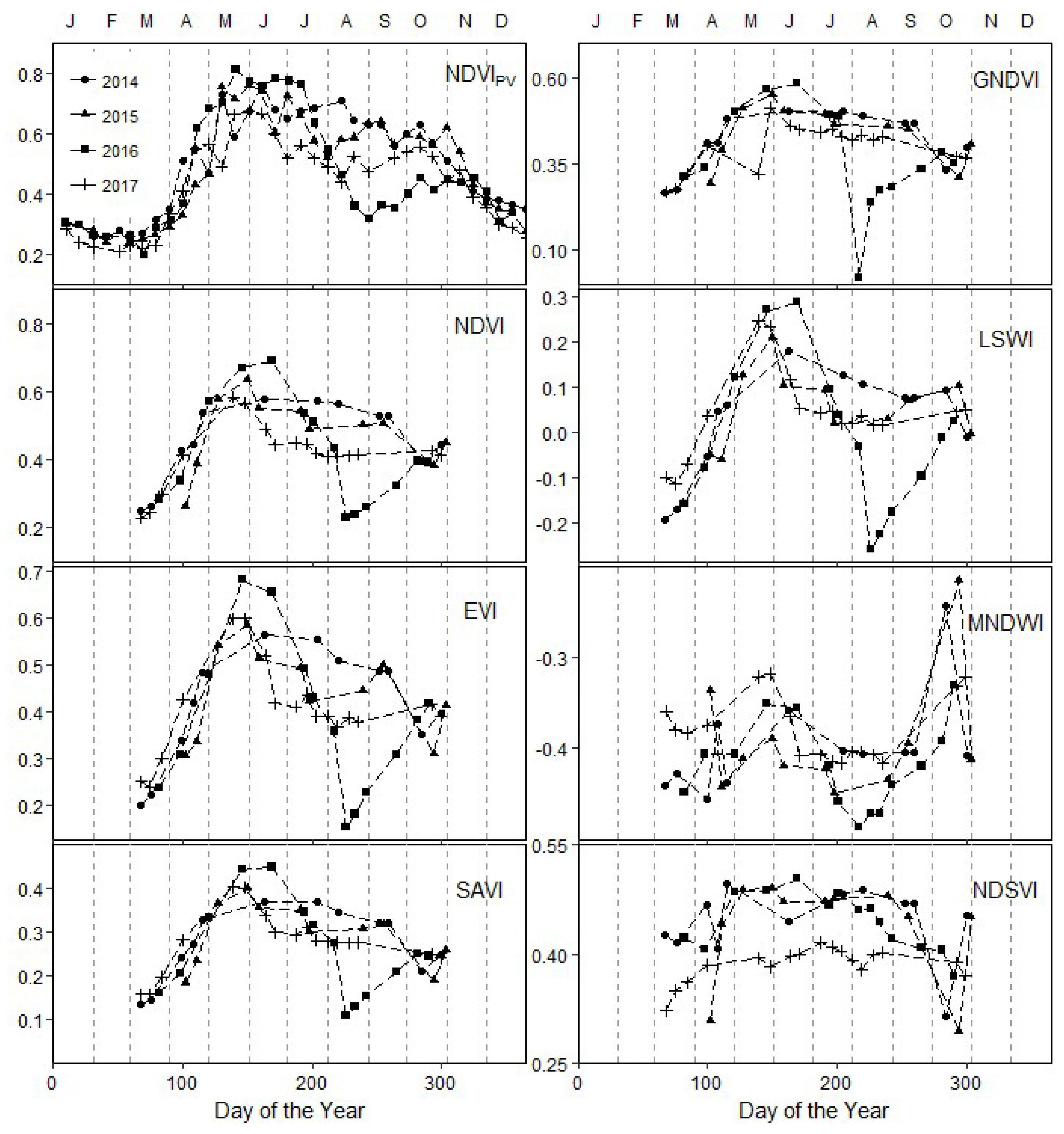
The temporal trends of the considered spectral vegetation indices are reported in Figure 3. All the vegetation indices that represent vegetation greenness (NDVI, EVI, SAVI and GNDVI) have quite similar trends. In addition, NDVI from the two different sources (Landsat and Proba-V) match quite well, with the difference that NDVIPV has slightly higher values than NDVI. All the vegetation indices increase from the beginning of the growing season, to reach a peak around end of May or beginning of June. After that, they start decreasing slowly for about 3 months. Around September, there is again a slight increase in the vegetation index. This last increase is better seen with NDVIPV especially in years 2016 and 2017.
Similar patterns in fluxes were visible every year: GPP shows some seasonality and has two peaks during the growing season, a high peak around end of May–beginning of June and a low peak in October. In between the two peaks, there is a period of low C uptake (lower GPP) values in July and August. Similar trends were visible in NEE and Reco. In fact, a strong correlation was observed between NEE and GPP during the growing season, both for midday and daily averages (r = 0.96 and 0.89 respectively).
The maximum values of VPD and Tair match the low GPP period. Rg, however, reaches its yearly peak earlier than VPD and Tair, somewhere between May and June. Precipitation data shows no real pattern of seasonality, as the distribution over the year seems quite random. However, less precipitation was observed in July and August in years 2016 and 2017.
The year 2016 shows an unusual trend, with a very low value recorded for some vegetation indices in August, due to a fire that occurred at that period. This unexpected disturbance was visible in GNDVI, NDVI, EVI, SAVI, LSWI and MNDWI, but less visible in NDVIPV and NDSVI.
LSWI is a water-related vegetation index, but it has a trend that is similar to the greenness-related vegetation indices. NDSVI, which is also a water-related vegetation index, does not decrease during June, July and August as MNDWI.

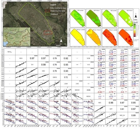
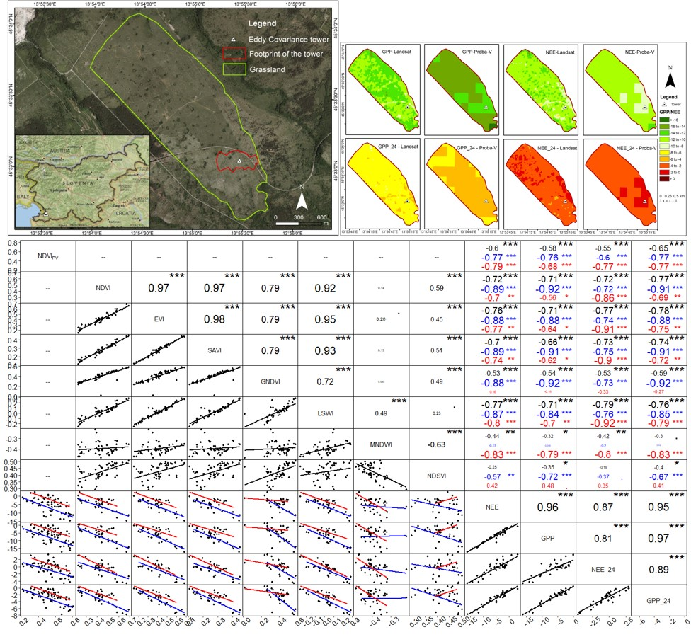
3.3. Correlation Charts of Fluxes and Vegetation Indices

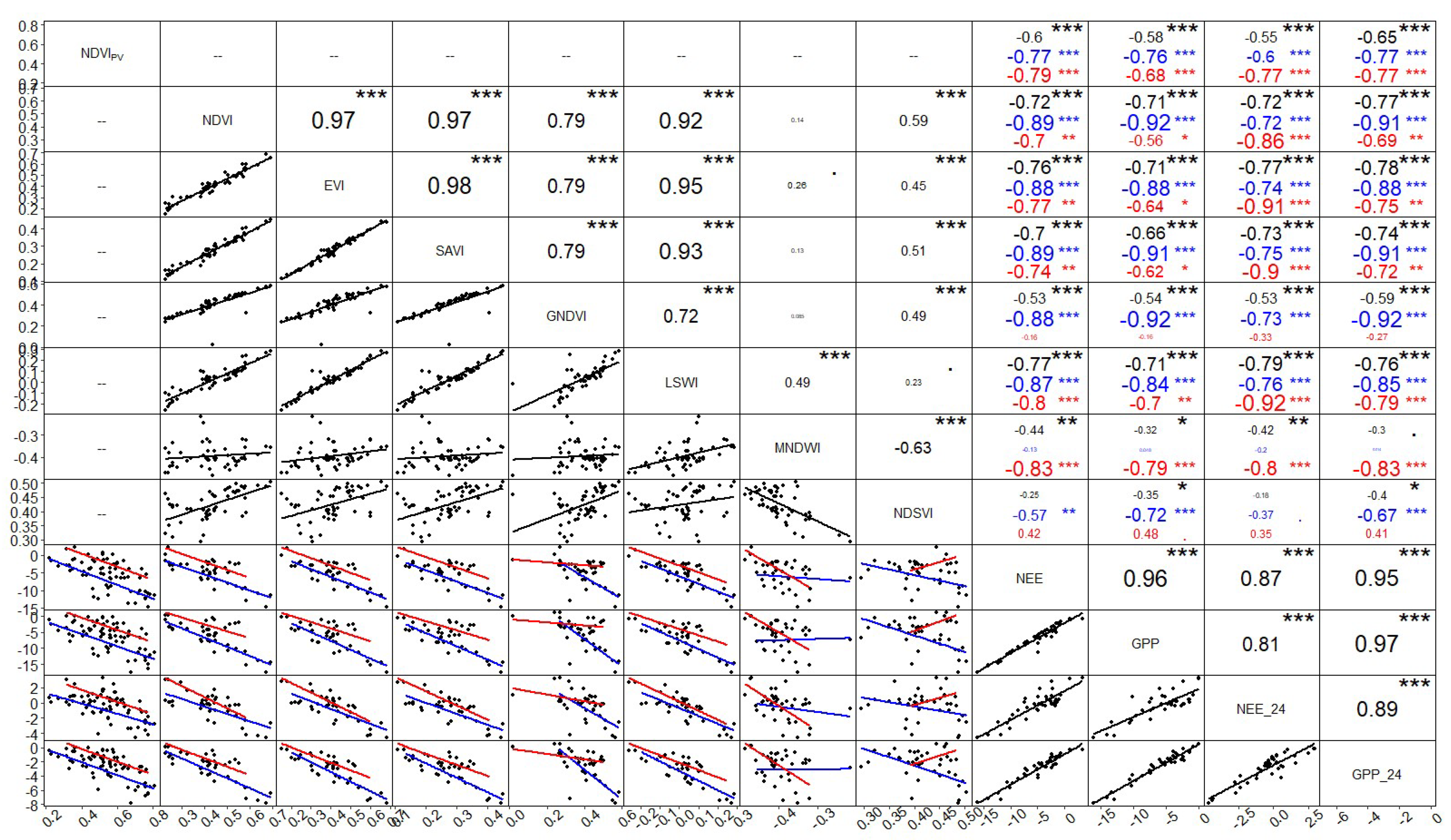
A correlation matrix of midday and daily aggregates of fluxes with all vegetation indices is shown in Figure 4. Correlations were evaluated for the wet phase (Figure 4, blue line), dry phase (red line) and the entire growing season. The good relationship among most vegetation indices, as previously mentioned, is confirmed by the high correlation coefficients. Only MNDWI and NDSVI were poorly correlated with the other vegetation indices.
On the correlation charts, only separate fit lines are shown (wet and dry phases) in order not to make the graphs overloaded (left bottom of the matrix). However, correlation coefficients were computed also for the whole season (values in black in the matrix). Low correlation coefficients were obtained for the whole season whereas the consideration of the two separate phases in the growing season resulted in higher correlation coefficients.
All the greenness-related VIs (NDVIPV, NDVI, EVI, SAVI and GNDVI) and LSWI gave higher correlation coefficients with GPP and midday NEE in the wet phase compared to the dry phase. In contrast, for daily NEE aggregates, the VIs, except GNDVI, gave a better correlation coefficient during the dry phase. MNDWI gave high correlation coefficients during the dry phase for GPP and NEE, both for midday and daily aggregates. NDSVI gave better correlation coefficients during the wet phase than the dry phase for GPP and NEE with both aggregates, but generally lower than correlation coefficients observed with other VIs.

3.4. Comparison of the Different Models

Values of accuracy metrics for the three models and for midday average fluxes are reported in Table 3. Similarly, Table 4 shows accuracy metrics for daily average fluxes. The values of these two tables directly reflect trends and correlation coefficients previously presented in Figure 4. No exceptions were found in our study, as high values of R2 corresponded always to low values of RMSE and AIC.
The best model for the entire growing season considering Landsat VIs was always obtained with LSWI for NEE and EVI for GPP in a direct correlation (model 1), either with midday or daily average fluxes. In contrast, NDVIPV gave lower R2 values in all models and for both aggregations of flux data (midday and daily) when the whole growing season was considered.
Overall, separate fits gave higher R2 and lower RMSE for all models than considering the whole growing season. For the wet phase, NDVI was the best predictor of midday aggregates for both GPP and NEE with all three model types. For daily aggregates, NDVI was the best vegetation index only in models 2 and 3 whereas in model 1, LSWI and GNDVI were the best vegetation indices for NEE and GPP respectively. For the dry phase, MNDWI was the best predictor of midday aggregates of GPP and NEE with all three model types. For daily aggregates, MNDWI was the best VI except in model 2 and model 1 with NEE, where LSWI gave the highest R2.
Midday fluxes gave higher R2 than daily fluxes during the wet phase for the model 1 (direct correlation carbon fluxes-VIs). However, during the dry phase (all models) and also the wet phase with models including PAR or Rg (2 and 3), daily fluxes gave higher R2 than midday fluxes.
The bootstrapped R2boot values were very similar to the R2 values, with very narrow 95% confidence intervals. The only time where the best results differ between R2 and R2boot was for midday estimate of NEE, which seems to be the best with MNDWI when considering R2 and LSWI if R2boot were considered instead.
Based on these accuracy metrics, the best regression models are presented in Table 5, according to the two aggregates (midday and daily), sources of vegetation indices (Landsat and Proba-V) and fluxes (GPP and NEE) for the two phases of the growing season. Direct correlation (model type 1) was found to be the best option for midday average fluxes, except for the estimation of GPP with NDVIPV during the wet phase, where the model type 2 was the best. For daily averages, however, the model type 1 performed better with NEE whereas model types 2 and 3 were the best for GPP.
During the wet phase, the best models obtained for GPP gave higher coefficients of determination (R2) compared to those obtained with NEE. The opposite was observed for the dry phase.
Based on the best models reported in Table 5, the Table 6 gives midday and daily estimates of GPP and NEE from NDVIPV data for the growing season (March to October) of the years 2014 to 2017. Average flux estimates of the four years are −711 g C m−2 growing season−1 and −199 g C m−2 growing season−1 for GPP and NEE respectively.

3.5. Flux Maps Using the Best Models

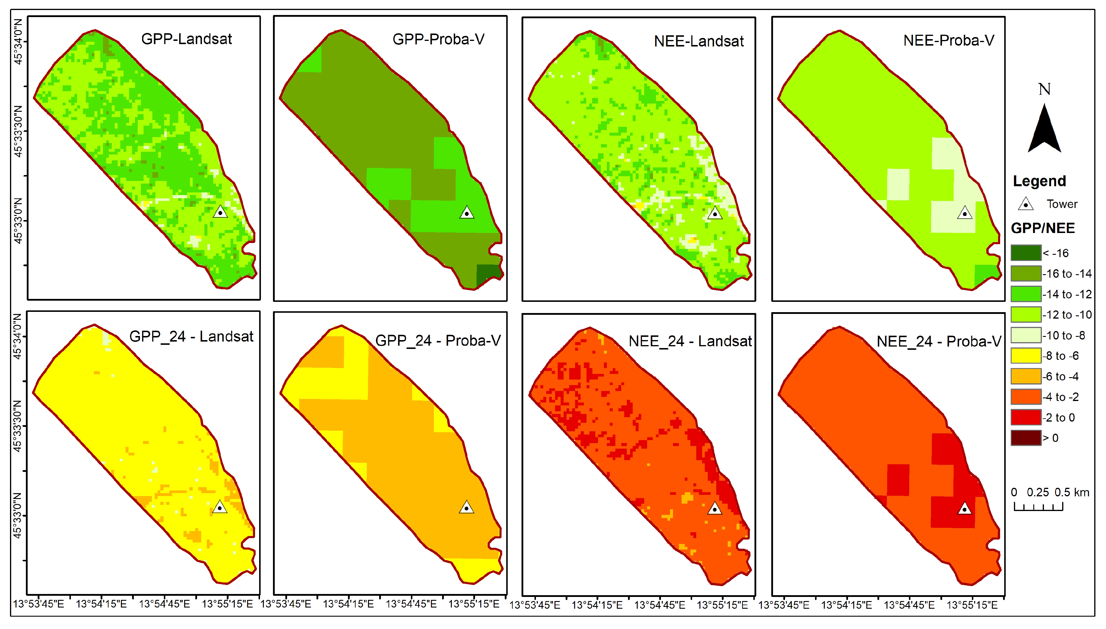
Figure 5 shows a map of GPP and NEE for the whole study area, computed based on the equations in 
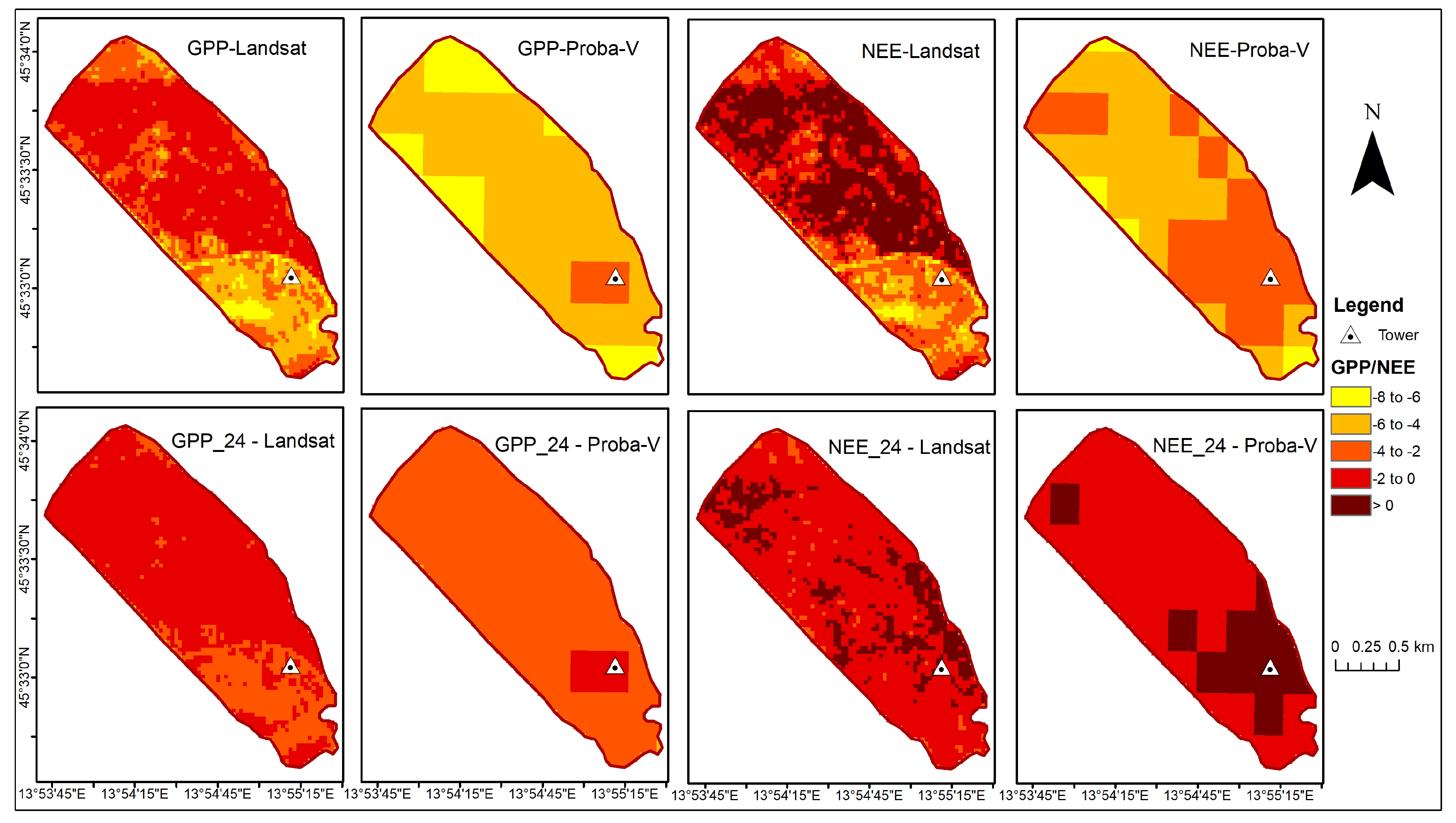
Table 5. These fluxes represent estimated averages for the periods 15 May 2017 to 19 May 2017 for Landsat and 11 May 2017 to 20 May 2017 for Proba-V. Similarly, Figure 6 shows estimated average of NEE and GPP for the periods 2 July 2017 to 6 July 2017 for Landsat and 1 July 2017 to 10 July 2017 for Proba-V. The dates were chosen to show an example for both wet and dry phases.
During the wet phase (Figure 5), GPP or NEE estimated from the two different sources of vegetation indices have similar spatial distributions in spite of their different spatial resolution. In the case of midday average fluxes, NEE and GPP seem to have the same distribution with differences only in their values. This is a consequence of the very good linear relationship that was found between midday GPP and NEE in our study. Daily fluxes, however, show more difference between NEE and GPP, as the correlation observed was not as good as that of midday fluxes.
During the dry phase (Figure 6), the spatial distribution of fluxes is quite different between flux estimates from the two sources of VI (Landsat and Proba-V), with the exception of estimates of daily aggregates of NEE, where the estimate from NDVIPV appears like a generalization of the estimate from LSWI.
A difference can be noticed between the wet and the dry phases: GPP estimates are very low during the dry phase, and the carbon balance (NEE estimates) became positive in some parts of the study area.

4. Discussion

In our study, the low C uptake observed during the period June to August with high VPD and Tair, and relatively lower precipitation confirmed that summer water stress is a major constraint in C sequestration for grasslands in the karst region characterized by shallow soils [36]. Regression models obtained demonstrated the ability of spectral vegetation indices to represent the impact of climate constraints on both NEE and GPP.

4.1. Performance of the Different Vegetation Indices

Overall, NDVI was the best predictor for the estimation of NEE and GPP during the wet phase of the growing season, reinforcing the conclusion of previous studies that NDVI is a suitable index for depicting photosynthetic C assimilation [9,64,65]. In addition, the best results obtained with NDVI instead of EVI or GNDVI suggest that the frequently reported issue of NDVI saturation was not observed in our study. Indeed, NDVI values observed are below the threshold of 0.8 reported for grasslands above which saturation has been observed [66,67]. On the other hand, the fact that greenness related vegetation indices were less performant when the entire growing season was considered is probably due to the influence of increased VPD on GPP and tissue water content in the karst grassland addressed by our study, during the dry phase. In fact, LSWI and MNDWI proved to be ideal for estimating fluxes during the dry period, confirming the fact that water-related vegetation indices are the best indicators of photosynthetic activity during dry periods, as they are more sensitive to water availability than the other vegetation indices [23]. NDSVI, which is also a water-related vegetation index, did not give as good results for the dry phase as LSWI and MNDWI. Other studies reported the low performance of NDSVI in depicting non-photosynthetic vegetation in a semi-arid grassland and a cropland [68,69], which is confirmed by the low performance observed in our study.
The two sources of vegetation indices (Landsat and Proba-V) could not really be compared, given that Landsat images were single date images whereas NDVIPV are 10 days composite data. In addition, the difference in the time step of aggregation of fluxes (10 days for NDVIPV and 5 days for Landsat vegetation indices) makes a comparison inappropriate. However, it should be noted that the highest correlation coefficient obtained with NDVIPV is generally lower than the one obtained with Landsat vegetation indices. This is probably due to the greater variability in fluxes and NDVIPV within the aggregation timeframe of the NDVIPV data (10 days).
The similarity in the correlation observed for most of the VIs with GPP and NEE is probably the consequence of the good relationship observed between the two variables, which often occurs when the analysis is focused on the growing season [29,30,31].
Despite the fire event that occurred in August 2016, we did not notice any outliers corresponding to that period in our regressions. This might be explained by the occurrence of the fire event towards the end of the dry phase, and the grasses recovered during the second part of the wet phase in September. Indeed, grasslands are known to recover quickly following a fire event [70].

4.2. Performance of the Different Models

In agreement with recent evidence [9,17], we observed an increase of model fitness when data were split into a dry and a wet phase, in contrast with the general agreement that LUE can be considered constant in grasslands along the whole growing season. Recent studies addressed this problem by attempting independent LUE estimations from the PRI and SIF [19,24]. Other models constrain LUE by decreasing a maximum value (LUEmax) with meteorological variables (scalars) [11]. In the present study, good results have been achieved by splitting the growing season into a wet and dry phases, reducing model input and further calculations.
The higher correlation coefficients observed between VIs and midday average fluxes compared to daily average fluxes during the wet phase could be due to the fact that most C uptake occur around midday during that phase of the growing season. During the dry phase however, depending on daily environmental conditions, there can be more variation in the midday average fluxes compared to daily averages. Hence during dry periods, daily averages showed more robust and higher correlations with VIs than midday averages. Overall, despite the differences observed, daily estimates were robust enough in our study to suggest their use instead of midday average flux estimates, being more representative of the total productivity of the ecosystem.
The validation of the models using the bootstrapping resampling method confirmed the assessment made with the regular accuracy metrics. The narrow 95% confidence intervals obtained for the R2boot reflects the low variability of the coefficient of determination obtained from the different bootstrapping samples.
From our carbon flux estimates, we could deduce that during the growing season, midday GPP represents over half of the whole day fluxes. NEE values are negative, which means that at least during the growing season, the grassland of our study area acts as a carbon sink. To our knowledge, there are no studies that estimated carbon fluxes in a karst grassland. However, the average GPP and NEE of −711 and −199 g C m−2 per growing season respectively are in range with estimates, of −867 and −132 g C m−2 per season respectively for GPP and NEE, obtained by [71] in a Mediterranean grassland.

4.3. GPP and NEE Maps

The use of regression models in our study for mapping GPP or NEE helped to appreciate the spatial variations in C uptake and C sequestration in a homogeneous area and estimate the contribution of grasslands. However, the spatial variability in C fluxes depended on the spatial variability of the vegetation indices. The obtained models should therefore be used only in homogenous environmental conditions.
Carbon fluxes maps obtained from NDVIPV appeared as a generalization of that obtained from Landsat derived VIs, which reflects the different spatial resolution of data from the two platforms. This suggests the possibility to rely on NDVIPV data for its availability, especially when a continuous estimation of carbon fluxes is needed over a certain period of time.
During drought periods, an ecosystem can quickly shift from carbon sink to source [72]. The difference observed in the maps of NEE between the wet and the dry phases illustrates this fact, since NEE values became positive during the dry phase, demonstrating the importance of comparing maps of the same area over time.

5. Conclusions

The main outcome of this study is an optimized model based on vegetation indices for estimating GPP (and NEE) in a karst grassland. Our results confirmed similar predicting power of NDVI and other VIs, even though greenness-related and water-related VIs were more adequate for the wet and the dry phases of the growing season, respectively. Finally, we demonstrated the usefulness of digital maps for an easy assessment and comparison of the spatial and temporal trends in the fluxes in the study area with possible practical application for local stakeholders.

Author Contributions

The six authors fully contributed in the research. S.C. and M.F. supervised the entire research; M.F., K.E., G.A. and A.P. collected field data; K.D.N. and M.F. conducted the data analysis; K.D.N. and S.C. prepared the original draft; All authors reviewed and edited the document.

Funding

This research was funded by the European Research Council (ERC) under the European Union’s Horizon 2020 research and innovation program under grant agreement No. 774234, and also by the Slovenian Research Agency, projects Z4-8217 and J4-9297 and research programmes P4-0107 and P4-0085. This work further benefited from the Erasmus Mundus MEDFOR (Mediterranean Forestry and Natural Resources Management) (520137-1-2011-1-PT-ERA MUNDUS-EMMC) fund.

Acknowledgments

The authors acknowledge the support of the project MEDSPEC (Monitoring gross primary productivity in Mediterranean oak woodlands through remote sensing and biophysical modelling (PTDC/AAG-MAA/3699/2014), and the research activities of the Forest Research Centre (PEst-OE/AGR/UI0239/2011) both funded by the Fundação para a Ciência e a Tecnologia, Ministry of Science and Education, Portugal.

Conflicts of Interest

The authors declare no conflict of interest.

References

  1. Mason, J.A.; Zanner, C.W. Grassland soils. In Encyclopedia of Soils in the Environment; Elsevier: Amsterdam, The Netherlands, 2005; pp. 138–145. ISBN 9780123485304. [Google Scholar]
  2. Scurlock, J.M.O.; Hall, D.O. The global carbon sink: A grassland perspective. Glob. Chang. Biol. 1998, 4, 229–233. [Google Scholar] [CrossRef]
  3. Buringh, P. Organic Carbon in Soils of the World. In The role of Terrestrial Vegetation in the Global Carbon Cycle: Measurement by Remote Sensing; Woodwell, G.M., Ed.; SCOPE 23; Wiley: Chichester, UK, 1984; pp. 41–109. [Google Scholar]
  4. Papale, D.; Reichstein, M.; Aubinet, M.; Canfora, E.; Bernhofer, C.; Kutsch, W.; Longdoz, B.; Rambal, S.; Valentini, R.; Vesala, T.; et al. Towards a standardized processing of Net Ecosystem Exchange measured with eddy covariance technique: Algorithms and uncertainty estimation. Biogeosciences 2006, 3, 571–583. [Google Scholar] [CrossRef]
  5. Burba, G.; Anderson, D. A Brief Practical Guide to Eddy Covariance Flux Measurements: Principles and Workflow Examples for Scientific and Industrial Applications; LI-COR Biosciences: Lincoln, NB, USA, 2010. [Google Scholar]
  6. Kirschbaum, M.U.F.; Eamus, D.; Gifford, R.M.; Roxburgh, S.H.; Sands, P.J. Definitions of Some Ecological Terms Commonly Used in Carbon Accounting. In Proceedings of the Net Ecosystem Exchange, Canberra, Australia, 18–20 April 2001; pp. 1–144. [Google Scholar]
  7. Aubinet, M.; Vesala, T.; Papale, D. Eddy Covariance A Practical Guide to Measurement and Data Analysis; Springer: New York, NY, USA, 2012; ISBN 9789400723504. [Google Scholar]
  8. Myneni, R.B.; Williams, D.L. On the relationship between FAPAR and NDVI. Remote Sens. Environ. 1994, 49, 200–211. [Google Scholar] [CrossRef]
  9. Nestola, E.; Calfapietra, C.; Emmerton, C.A.; Wong, C.Y.S.; Thayer, D.R.; Gamon, J.A. Monitoring grassland seasonal carbon dynamics, by integrating MODIS NDVI, proximal optical sampling, and eddy covariance measurements. Remote Sens. 2016, 8, 25. [Google Scholar] [CrossRef]
  10. Running, S.W.; Nemani, R.R.; Heinsch, F.A.; Zhao, M.; Reeves, M.; Hashimoto, H. A Continuous Satellite-Derived Measure of Global Terrestrial Primary Production. Bioscience 2004, 54, 547. [Google Scholar] [CrossRef] [Green Version]
  11. Yuan, W.; Cai, W.; Xia, J.; Chen, J.; Liu, S.; Dong, W.; Merbold, L.; Law, B.; Arain, A.; Beringer, J.; et al. Global comparison of light use efficiency models for simulating terrestrial vegetation gross primary production based on the LaThuile database. Agric. For. Meteorol. 2014, 192–193, 108–120. [Google Scholar] [CrossRef]
  12. Zhou, X.; Zhu, Q.; Tang, S.; Chen, X.; Wu, M. Interception of PAR and relationship between FPAR and LAI in summer maize canopy. In Proceedings of the IEEE International Geoscience and Remote Sensing Symposium, Toronto, ON, Canada, 24–28 June 2002; Volume 6, pp. 3252–3254. [Google Scholar]
  13. Yan, W.; Hu, Z.; Zhao, Y.; Zhang, X.; Fan, Y.; Shi, P. Modeling Net Ecosystem Carbon Exchange of Alpine Grasslands with a Satellite-Driven Model. PLoS ONE 2015, 10, e0122486. [Google Scholar] [CrossRef] [PubMed]
  14. Zhou, Y.; Zhang, L.; Xiao, J.; Chen, S.; Kato, T.; Zhou, G. A comparison of satellite-derived vegetation indices for approximating gross primary productivity of grasslands. Rangel. Ecol. Manag. 2014, 67, 9–18. [Google Scholar] [CrossRef]
  15. Rocha, A.V.; Shaver, G.R. Advantages of a two band EVI calculated from solar and photosynthetically active radiation fluxes. Agric. For. Meteorol. 2009, 149, 1560–1563. [Google Scholar] [CrossRef]
  16. Gitelson, A.A.; Kaufman, Y.J.; Merzlyak, M.N. Use of a green channel in remote sensing of global vegetation from EOS-MODIS. Remote Sens. Environ. 1996, 58, 289–298. [Google Scholar] [CrossRef]
  17. Cerasoli, S.; Campagnolo, M.; Faria, J.; Nogueira, C.; Caldeira, M.D.C. On estimating the gross primary productivity of Mediterranean grasslands under different fertilization regimes using vegetation indices and hyperspectral reflectance. Biogeosciences 2018, 15, 5455–5471. [Google Scholar] [CrossRef]
  18. Jovanović, D.; Govedarica, M.; Sabo, F.; Važić, R.; Popović, D. Impact analysis of pansharpening Landsat ETM+, Landsat OLI, WorldView-2, and Ikonos images on vegetation indices. In Proceedings of the Fourth International Conference on Remote Sensing and Geoinformation of the Environment (RSCy2016), Paphos, Cyprus, 4–6 April 2016; Themistocleous, K., Hadjimitsis, D.G., Michaelides, S., Papadavid, G., Eds.; 2016; Volume 9688, p. 10. [Google Scholar]
  19. Rossini, M.; Cogliati, S.; Meroni, M.; Migliavacca, M.; Galvagno, M.; Busetto, L.; Cremonese, E.; Julitta, T.; Siniscalco, C.; Morra, U.; et al. Remote sensing-based estimation of gross primary production in a subalpine grassland. Biogeosciences 2012, 9, 2565–2584. [Google Scholar] [CrossRef] [Green Version]
  20. Sakowska, K.; Vescovo, L.; Marcolla, B.; Juszczak, R.; Olejnik, J.; Gianelle, D. Monitoring of carbon dioxide fluxes in a subalpine grassland ecosystem of the Italian Alps using a multispectral sensor. Biogeosciences 2014, 11, 4695–4712. [Google Scholar] [CrossRef] [Green Version]
  21. John, R.; Chen, J.; Lu, N.; Guo, K.; Liang, C.; Wei, Y.; Noormets, A.; Ma, K.; Han, X. Predicting plant diversity based on remote sensing products in the semi-arid region of Inner Mongolia. Remote Sens. Environ. 2008, 112, 2018–2032. [Google Scholar] [CrossRef]
  22. Hill, M.J. Vegetation index suites as indicators of vegetation state in grassland and savanna: An analysis with simulated SENTINEL 2 data for a North American transect. Remote Sens. Environ. 2013, 137, 94–111. [Google Scholar] [CrossRef]
  23. Bajgain, R.; Xiao, X.; Wagle, P.; Basara, J.; Zhou, Y. Sensitivity analysis of vegetation indices to drought over two tallgrass prairie sites. ISPRS J. Photogramm. Remote Sens. 2015, 108, 151–160. [Google Scholar] [CrossRef]
  24. Wagle, P.; Zhang, Y.; Jin, C.; Xiao, X. Comparison of solar-induced chlorophyll fluorescence, light-use efficiency, and process-based GPP models in maize. Ecol. Appl. 2016, 26, 1211–1222. [Google Scholar] [CrossRef]
  25. Sims, D.A.; Rahman, A.F.; Cordova, V.D.; El-Masri, B.Z.; Baldocchi, D.D.; Bolstad, P.V.; Flanagan, L.B.; Goldstein, A.H.; Hollinger, D.Y.; Misson, L.; et al. A new model of gross primary productivity for North American ecosystems based solely on the enhanced vegetation index and land surface temperature from MODIS. Remote Sens. Environ. 2008, 112, 1633–1646. [Google Scholar] [CrossRef]
  26. Goerner, A.; Reichstein, M.; Tomelleri, E.; Hanan, N.; Rambal, S.; Papale, D.; Dragoni, D.; Schmullius, C. Remote sensing of ecosystem light use efficiency with MODIS-based PRI. Biogeosciences 2011, 8, 189–202. [Google Scholar] [CrossRef]
  27. Li, Z.; Yu, G.; Xiao, X.; Li, Y.; Zhao, X.; Ren, C.; Zhang, L.; Fu, Y. Modeling gross primary production of alpine ecosystems in the Tibetan Plateau using MODIS images and climate data. Remote Sens. Environ. 2007, 107, 510–519. [Google Scholar] [CrossRef]
  28. Gilmanov, T.; Tieszen, L.L.; Wylie, B.K.; Flanagan, L.B.; Frank, A.B.; Haferkamp, M.R.; Meyers, T.P.; Morgan, J.A. Integration of CO2 flux and remotely-sensed data for primary production and ecosystem respiration analyses in the Northern Great Plains: Potential for quantitative spatial extrapolation. Glob. Ecol. Biogeogr. 2005, 14, 271–292. [Google Scholar] [CrossRef]
  29. Baldocchi, D.D. “Breathing” of the terrestrial biosphere: Lessons learned from a global network of carbon dioxide flux measurement systems. Aust. J. Bot. 2008, 56, 1. [Google Scholar] [CrossRef]
  30. Baldocchi, D.D.; Sturtevant, C. Fluxnet contributors Does day and night sampling reduce spurious correlation between canopy photosynthesis and ecosystem respiration? Agric. For. Meteorol. 2015, 207, 117–126. [Google Scholar] [CrossRef]
  31. Ma, S.; Baldocchi, D.D.; Wolf, S.; Verfaillie, J. Slow ecosystem responses conditionally regulate annual carbon balance over 15 years in Californian oak-grass savanna. Agric. For. Meteorol. 2016, 228–229, 252–264. [Google Scholar] [CrossRef]
  32. Gabrovšek, K. People with Nature, Nature for People—Biodiversity is Our Life; Institute of the Republic of Slovenia for Nature Conservation: Ljubljana, Slovenia, 2010. [Google Scholar]
  33. Ferlan, M. The Use of Micro-Meteorological Methods for the Monitoring of the Carbon Fluxes in Karst Ecosystems. Ph.D. Thesis, University of Ljubljana, Ljubljana, Slovenia, 2013. [Google Scholar]
  34. Knez, M.; Petrič, M.; Slabe, T.; Šebela, S. The Beka-Ocizla Cave System: Karstological Railway Planning in Slovenia; Springer: New York, NY, USA, 2015; ISBN 9783319044552. [Google Scholar]
  35. EARS Environmental Agency of the Republic of Slovenia. Available online: http://meteo.arso.gov.si (accessed on 1 March 2019).
  36. Ferlan, M.; Alberti, G.; Eler, K.; Batič, F.; Miglietta, F.; Zaldei, A.; Simončič, P. Comparing carbon fluxes between different stages of secondary succession of a karst grassland. Agric. Ecosyst. Environ. 2011, 140, 199–207. [Google Scholar] [CrossRef]
  37. Schuepp, P.H.; Leclerc, M.Y.; MacPherson, J.I.; Desjardins, R.L. Footprint prediction of scalar fluxes from analytical solutions of the diffusion equation. Boundary-Layer Meteorol. 1990, 50, 355–373. [Google Scholar] [CrossRef]
  38. Aubinet, M.; Grelle, A.; Ibrom, A.; Rannik, Ü.; Moncrieff, J.; Foken, T.; Kowalski, A.S.; Martin, P.H.; Berbigier, P.; Bernhofer, C.; et al. Estimates of the Annual Net Carbon and Water Exchange of Forests: The EUROFLUX Methodology. Adv. Ecol. Res. 1999, 30, 113–175. [Google Scholar]
  39. Webb, E.K.; Pearman, G.I.; Leuning, R. Correction of flux measurements for density effects due to heat and water vapour transfer. Q. J. R. Meteorol. Soc. 1980, 106, 85–100. [Google Scholar] [CrossRef]
  40. Burba, G.; Mcdermitt, D.K.; Grelle, A.; Anderson, D.J.; Xu, L. Addressing the influence of instrument surface heat exchange on the measurements of CO2 flux from open-path gas analyzers. Glob. Chang. Biol. 2008, 14, 1854–1876. [Google Scholar] [CrossRef]
  41. University of Edinburgh EdiRe Software for Micrometeorological Applications(App. Note Code: 3C-R); Campbell Scientific: Logan, UT, USA, 1999.
  42. Foken, T.; Wichura, B. Tools for quality assessment of surface-based flux measurements. Agric. For. Meteorol. 1996, 78, 83–105. [Google Scholar] [CrossRef]
  43. Meek, D.W.; Hatfield, J.L.; Howell, T.A.; Idso, S.B.; Reginato, R.J. A Generalized Relationship between Photosynthetically Active Radiation and Solar Radiation1. Agron. J. 1984, 76, 939–945. [Google Scholar] [CrossRef]
  44. Lasslop, G.; Reichstein, M.; Papale, D.; Richardson, A.D.; Arneth, A.; Barr, A.; Stoy, P.; Wohlfahrt, G. Separation of net ecosystem exchange into assimilation and respiration using a light response curve approach: Critical issues and global evaluation. Glob. Chang. Biol. 2010, 16, 187–208. [Google Scholar] [CrossRef]
  45. CGLSP Copernicus Global Land Service Portal. Available online: http://land.copernicus.vgt.vito.be/PDF/portal/Application.html#Browse;Root=513186;Collection=1000063;Time=NORMAL,NORMAL,-1,,,-1,, (accessed on 20 December 2017).
  46. USGS United States Geological Survey. Available online: https://glovis.usgs.gov/ (accessed on 5 January 2018).
  47. Saranya, M. Cloud Removal from Satellite Images Using Information Cloning. Int. J. Comput. Sci. Mob. Comput. 2014, 32, 681–688. [Google Scholar]
  48. Sun, L.; Mi, X.; Wei, J.; Wang, J.; Tian, X.; Yu, H.; Gan, P. A cloud detection algorithm-generating method for remote sensing data at visible to short-wave infrared wavelengths. ISPRS J. Photogramm. Remote Sens. 2017, 124, 70–88. [Google Scholar] [CrossRef]
  49. USGS United States Geological Survey. Available online: https://earthexplorer.usgs.gov/ (accessed on 1 March 2019).
  50. Chavez, P.S.J. Image-based atmospheric corrections—Revisited and improved. Photogramm. Eng. Remote Sens. 1996, 62, 1025–1036. [Google Scholar]
  51. R Core Team R: A Language and Environment for Statistical Computing. R Foundation for Statistical Computing. Available online: http://www.r-project.org/ (accessed on 1 March 2019).
  52. Rouse, J.W.; Haas, R.H.; Schell, J.A.; Deering, D.W. Monitoring vegetation systems in the Great Plains with ERTS. In Proceedings of the 3rd Earth Resources Satellite-1 Symposium (NASA SP-351), Washington, DC, USA, 10–14 December 1973. [Google Scholar]
  53. Huete, A.; Didan, K.; Miura, T.; Rodriguez, E.P.; Gao, X.; Ferreira, L.G. Overview of the radiometric and biophysical performance of the MODIS vegetation indices. Remote Sens. Environ. 2002, 83, 195–213. [Google Scholar] [CrossRef]
  54. Huete, A.R. A soil-adjusted vegetation index (SAVI). Remote Sens. Environ. 1988, 25, 295–309. [Google Scholar] [CrossRef]
  55. Xiao, X.; Boles, S.; Liu, J.; Zhuang, D.; Frolking, S.; Li, C.; Salas, W.; Moore, B. Mapping paddy rice agriculture in southern China using multi-temporal MODIS images. Remote Sens. Environ. 2005, 95, 480–492. [Google Scholar] [CrossRef]
  56. Xu, H. Modification of normalised difference water index (NDWI) to enhance open water features in remotely sensed imagery. Int. J. Remote Sens. 2006, 27, 3025–3033. [Google Scholar] [CrossRef]
  57. Sulman, B.N.; Roman, D.T.; Yi, K.; Wang, L.; Phillips, R.P.; Novick, K.A. High atmospheric demand for water can limit forest carbon uptake and transpiration as severely as dry soil. Geophys. Res. Lett. 2016, 43, 9686–9695. [Google Scholar] [CrossRef]
  58. Will, R.E.; Wilson, S.M.; Zou, C.B.; Hennessey, T.C. Increased vapor pressure deficit due to higher temperature leads to greater transpiration and faster mortality during drought for tree seedlings common to the forest-grassland ecotone. New Phytol. 2013, 200, 366–374. [Google Scholar] [CrossRef] [PubMed] [Green Version]
  59. Maherali, H.; Maherali, H.; Johnson, H.B.; Jackson, R.B. Stomatal sensitivity to vapour pressure difference over a subambient to elevated CO2 gradient in a C3/C4 grassland. Plant Cell Environ. 2003, 26, 1297–1306. [Google Scholar] [CrossRef]
  60. Anderson, L.J.; Maherali, H.; Johnson, H.B.; Polley, H.W.; Jackson, R.B. Gas exchange and photosynthetic acclimation over subambient to elevated CO2 in a C3-C4 grassland. Glob. Chang. Biol. 2001, 7, 693–707. [Google Scholar] [CrossRef] [Green Version]
  61. Richter, K.; Atzberger, C.; Hank, T.B.; Mauser, W. Derivation of biophysical variables from Earth observation data: Validation and statistical measures. J. Appl. Remote Sens. 2012, 6, 063557. [Google Scholar] [CrossRef]
  62. Tagesson, T.; Ardö, J.; Cappelaere, B.; Kergoat, L.; Abdi, A.; Horion, S.; Fensholt, R. Modelling spatial and temporal dynamics of gross primary production in the Sahel from earth-observation-based photosynthetic capacity and quantum efficiency. Biogeosciences 2017, 14, 1333–1348. [Google Scholar] [CrossRef]
  63. Bagaram, M.; Giuliarelli, D.; Chirici, G.; Giannetti, F.; Barbati, A. UAV Remote Sensing for Biodiversity Monitoring: Are Forest Canopy Gaps Good Covariates? Remote Sens. 2018, 10, 1397. [Google Scholar]
  64. Gamon, J.A.; Field, C.B.; Goulden, M.L.; Griffin, K.L.; Hartley, A.E.; Joel, G.; Penuelas, J.; Valentini, R. Relationships Between NDVI, Canopy Structure, and Photosynthesis in Three Californian Vegetation Types. Ecol. Appl. 1995, 5, 28–41. [Google Scholar] [CrossRef] [Green Version]
  65. Myneni, R.B.; Hall, F.G.; Sellers, P.J.; Marshak, A.L. The interpretation of spectral vegetation indexes. IEEE Trans. Geosci. Remote Sens. 1995, 33, 481–486. [Google Scholar] [CrossRef]
  66. Gianelle, D.; Vescovo, L.; Marcolla, B.; Manca, G.; Cescatti, A. Ecosystem carbon fluxes and canopy spectral reflectance of a mountain meadow. Int. J. Remote Sens. 2009, 30, 435–449. [Google Scholar] [CrossRef]
  67. Vescovo, L.; Wohlfahrt, G.; Balzarolo, M.; Pilloni, S.; Sottocornola, M.; Rodeghiero, M.; Gianelle, D. New spectral vegetation indices based on the near-infrared shoulder wavelengths for remote detection of grassland phytomass. Int. J. Remote Sens. 2011, 33, 2178–2195. [Google Scholar] [CrossRef] [PubMed] [Green Version]
  68. Sonmez, N.K.; Slater, B. European Journal of Remote Sensing Measuring Intensity of Tillage and Plant Residue Cover Using Remote Sensing. Eur. J. Remote Sens. 2016, 49, 121–135. [Google Scholar] [CrossRef]
  69. Li, Z.; Guo, X. Non-photosynthetic vegetation biomass estimation in semiarid Canadian mixed grasslands using ground hyperspectral data, Landsat 8 OLI, and Sentinel-2 images. Int. J. Remote Sens. 2018, 39, 6893–6913. [Google Scholar] [CrossRef]
  70. Keeley, J.E.; Keeley, S.C. Postfire Recovery of California Coastal Sage Scrub. Source Am. Midl. Nat. 1984, 111, 105–117. [Google Scholar] [CrossRef]
  71. Xu, L.; Baldocchi, D.D. Seasonal variation in carbon dioxide exchange over a Mediterranean annual grassland in California. Agric. For. Meteorol. 2004, 123, 79–96. [Google Scholar] [CrossRef] [Green Version]
  72. Lei, T.; Pang, Z.; Wang, X.; Li, L.; Fu, J.; Kan, G.; Zhang, X.; Ding, L.; Li, J.; Huang, S.; et al. Drought and Carbon Cycling of Grassland Ecosystems under Global Change: A Review. Water 2016, 8, 460. [Google Scholar] [CrossRef]
Figure 1. Study area, a karst grassland.
Remotesensing 11 00649 g001
Figure 2. Daily average of NEE (a) (the red line represents the moving average of daily NEE with a 20 days window); Reco and GPP (b) (the green and red lines represent the moving average of daily GPP and Reco, respectively; 30 min average of VPD (c), Tair (d), Rg (e) and total daily precipitation (f) recorded between 2014 and 2017 at the study site.
Remotesensing 11 00649 g002
Figure 3. Temporal profile of vegetation indices calculated in this study (see Table 2). Different symbols represent different years.
Remotesensing 11 00649 g003
Figure 4. Correlation charts between fluxes and vegetation indices. Values in black, blue and red represent Pearson correlation coefficients for a single fit, the wet phase (VPD ≤ 1500 Pa) and the dry phase (VPD > 1500 Pa), respectively. The remark “_24” is used to distinguish daily average fluxes from midday average fluxes. *, **, *** indicates correlations significant at p < 0.05; p < 0.01 and p < 0.001, respectively.
Remotesensing 11 00649 g004
Figure 5. Maps of average midday and daily GPP and NEE estimates for the periods 15 May 2017 to 19 May 2017 (for Landsat) and 11 May 2017 to 20 May 2017 (for Proba-V), using the best models obtained for the wet phase (Table 5). The remark “_24” is used to distinguish daily from midday average fluxes.
Remotesensing 11 00649 g005
Figure 6. Maps of average midday and daily GPP and NEE estimates for the periods 2 July 2017 to 6 July 2017 (for Landsat) and 1 July 2017 to 10 July 2017 (for Proba-V), using the best models obtained for the dry phase (Table 5). The remark “_24” is used to distinguish daily from midday average fluxes.
Remotesensing 11 00649 g006
Table 1. Spectral range of Landsat and Proba-V bands.
NameLandsat Range (µm)Proba-V Range (µm)
Ultra Blue (coastal/aerosol)Band 1 (0.435–0.451)
BlueBand 2 (0.452–0.512)Band 1 (0.438–0.486)
GreenBand 3 (0.533–0.590)
RedBand 4 (0.636–0.673)Band 2 (0.615–0.696)
Near Infrared (NIR)Band 5 (0.851–0.879)Band 3 (0.772–0.914)
Shortwave Infrared (SWIR) 1Band 6 (1.566–1.651)Band 4 (1.564–1.634)
Shortwave Infrared (SWIR) 2Band 7 (2.107–2.294)
PanchromaticBand 8 (0.503–0.676)
CirrusBand 9 (1.363–1.384)
Thermal Infrared (TIRS) 1Band 10 (10.60–11.19
Thermal Infrared (TIRS) 2Band 11 (11.50–12.51)
Table 2. Vegetation indices adopted for this study.
SatelliteIndexFormulaReference
Proba-VNDVIPVNDVIPV = (b3 − b2)/(b2 + b3)[52]
Landsat 8NDVINDVI = (b5 − b4)/(b5 + b4)[52]
Landsat 8GNDVIGNDVI = (b5 − b3)/(b5 + b3)[16]
Landsat 8EVIEVI = (2.5*(b5 − b4))/(b5 + 6*b4 − 7.5*b2 + 1)[53]
Landsat 8NDSVINDSVI = (b6 − b4)/(b6 + b4)[21]
Landsat 8SAVISAVI = ((1 + L)(b5 − b4))/(b5 + b4 + L)[54]
Landsat 8LSWILSWI = (b5 − b6)/(b5 + b6)[55]
Landsat 8MNDWIMNDWI = (b3 − b6)/(b3 + b6)[56]
L is a constant dependent on the vegetation cover and takes values from 0 (for very green vegetation) to 1 (areas with no green vegetation), assumed 0.5 here, b1 to b6 represent band numbers defined in Table 1.
Table 3. GPP~VIs and NEE~VIs regression accuracy metrics (R2, R2boot, RMSE, AIC) obtained using only midday fluxes.
R2R2bootRMSEAIC
ModelFluxVIsSingleWetDrySingleWetDrySingleWetDrySingleWetDry
1 NEENDVIPV0.360.590.620.36 ± 0.000.6 ± 0.010.63 ± 0.013.342.511.72172.8381.4034.40
Flux = a*VI + b NDVI0.520.800.490.51 ± 0.010.79 ± 0.000.53 ± 0.012.871.682.6788.4630.9631.54
EVI0.580.780.590.55 ± 0.010.77 ± 0.010.64 ± 0.012.701.752.4083.6033.0528.50
SAVI0.480.790.550.46 ± 0.010.78 ± 0.010.61 ± 0.012.991.732.5191.7132.5229.76
GNDVI0.290.780.030.28 ± 0.010.77 ± 0.010.17 ± 0.013.521.763.68104.7733.3240.49
LSWI0.590.750.640.56 ± 0.010.74 ± 0.010.69 ± 0.012.681.882.2382.9636.7326.52
MNDWI0.190.020.690.19 ± 0.010.03 ± 0.000.66 ± 0.013.743.722.09109.6072.3124.68
NDSVI0.060.330.180.1 ± 0.010.4 ± 0.010.2 ± 0.014.043.073.38115.7362.3538.14
GPPNDVIPV0.330.580.460.34 ± 0.000.58 ± 0.010.48 ± 0.013.532.532.47180.5682.1054.57
NDVI0.500.850.320.5 ± 0.010.85 ± 0.000.34 ± 0.012.811.422.8384.4821.6533.17
EVI0.510.770.410.5 ± 0.010.77 ± 0.010.42 ± 0.012.781.742.6483.6231.8331.18
SAVI0.440.820.380.44 ± 0.010.82 ± 0.000.4 ± 0.012.971.542.7188.8125.6431.88
GNDVI0.300.850.020.31 ± 0.010.85 ± 0.000.15 ± 0.013.321.433.3997.6922.0438.19
LSWI0.500.710.480.49 ± 0.010.7 ± 0.010.49 ± 0.012.801.992.4784.2938.3329.29
MNDWI0.100.000.630.12 ± 0.010.03 ± 0.000.59 ± 0.013.763.672.10107.2468.9624.77
NDSVI0.120.520.230.15 ± 0.010.54 ± 0.010.27 ± 0.013.712.543.01106.2350.5334.81
2GPPNDVIPV0.100.730.370.11 ± 0.000.73 ± 0.010.38 ± 0.014.102.032.67201.5763.6158.99
GPP = a*(VI*Rg) + b NDVI0.190.810.190.2 ± 0.010.8 ± 0.000.22 ± 0.013.561.613.10103.0727.9235.66
EVI0.220.750.260.23 ± 0.010.74 ± 0.010.28 ± 0.013.501.822.95101.6433.9634.32
SAVI0.180.770.240.19 ± 0.010.76 ± 0.010.27 ± 0.013.601.762.99103.8332.3034.67
GNDVI0.100.730.010.12 ± 0.010.72 ± 0.010.12 ± 0.013.751.923.41107.1136.5538.39
LSWI0.480.740.470.47 ± 0.010.72 ± 0.010.47 ± 0.012.851.892.5185.6435.7129.76
MNDWI0.030.220.610.05 ± 0.000.23 ± 0.010.56 ± 0.013.903.252.13110.1562.9025.21
NDSVI0.010.550.130.03 ± 0.000.56 ± 0.010.17 ± 0.013.942.453.20110.9248.8336.53
3GPPNDVIPV0.110.730.450.13 ± 0.010.72 ± 0.010.46 ± 0.014.452.072.49212.8864.9755.10
GPP=LUE*(a*VI+b)*Rg NDVI0.260.840.250.27 ± 0.010.84 ± 0.000.28 ± 0.013.751.672.98107.0329.7234.58
EVI0.260.760.330.28 ± 0.010.76 ± 0.010.34 ± 0.013.721.922.84106.4136.7133.24
SAVI0.180.770.310.2 ± 0.010.77 ± 0.010.33 ± 0.013.921.902.87110.4836.0333.52
GNDVI0.110.800.010.14 ± 0.010.8 ± 0.010.12 ± 0.014.101.813.46114.0133.8038.73
LSWI0.270.740.400.28 ± 0.010.73 ± 0.010.41 ± 0.013.681.992.67105.6938.3231.45
MNDWI0.080.260.530.12 ± 0.010.3 ± 0.010.49 ± 0.013.903.152.38110.0861.4528.26
NDSVI0.030.670.180.07 ± 0.000.68 ± 0.010.22 ± 0.014.242.133.13116.6941.8035.92
In Table 3, for Landsat VIs, the best regression results for each model are highlighted in bold for the whole growing season (single) and for wet and dry periods. For Proba-V, the best regressions from all 3 models for NEE and GPP are highlighted for single, wet and dry.
Table 4. GPP~VIs and NEE~VIs regression accuracy metrics (R2, R2boot, RMSE, AIC) obtained using daily fluxes.
R2R2bootRMSEAIC
ModelFluxVIsSingleWetDrySingleWetDrySingleWetDrySingleWetDry
1NEENDVIPV0.300.360.590.3 ± 0.000.37 ± 0.010.59 ± 0.011.451.420.8055.8633.36−8.48
Flux = a*VI + b NDVI0.520.520.740.5 ± 0.010.5 ± 0.010.74 ± 0.011.231.210.8520.7013.92−0.61
EVI0.590.550.820.56 ± 0.010.51 ± 0.010.82 ± 0.011.131.170.7113.8012.31−5.69
SAVI0.540.570.810.52 ± 0.010.53 ± 0.010.82 ± 0.011.201.150.7418.9811.19−4.61
GNDVI0.280.530.110.3 ± 0.010.5 ± 0.010.26 ± 0.021.491.201.5836.8513.4616.79
LSWI0.620.580.860.61 ± 0.010.55 ± 0.010.85 ± 0.011.081.130.6310.5210.19−8.72
MNDWI0.180.040.640.17 ± 0.010.03 ± 0.000.6 ± 0.011.601.711.0042.4131.894.02
NDSVI0.030.140.130.06 ± 0.000.2 ± 0.010.16 ± 0.011.731.621.5649.1829.0716.48
GPPNDVIPV0.430.600.590.43 ± 0.000.59 ± 0.010.6 ± 0.011.411.180.9051.7717.58−1.92
NDVI0.590.820.470.61 ± 0.010.82 ± 0.000.5 ± 0.011.090.711.0711.18−12.885.79
EVI0.620.780.570.62 ± 0.010.77 ± 0.000.59 ± 0.011.060.800.969.02−7.372.98
SAVI0.540.830.520.56 ± 0.010.82 ± 0.000.56 ± 0.011.160.711.0115.93−13.464.33
GNDVI0.350.840.070.4 ± 0.010.84 ± 0.000.25 ± 0.021.390.681.4130.31−15.2713.69
LSWI0.580.730.620.61 ± 0.010.72 ± 0.010.65 ± 0.011.110.880.9012.36−2.341.08
MNDWI0.090.000.690.11 ± 0.010.02 ± 0.000.65 ± 0.011.641.700.8243.3930.47−1.55
NDSVI0.160.460.170.16 ± 0.010.46 ± 0.010.2 ± 0.011.571.251.3440.2715.2812.15
2GPPNDVIPV0.190.780.520.2 ± 0.000.78 ± 0.010.52 ± 0.011.670.870.9875.59−7.602.61
GPP=a*(VI*Rg)+b NDVI0.300.850.320.33 ± 0.010.84 ± 0.000.35 ± 0.011.430.661.2132.78−16.999.37
EVI0.340.810.400.37 ± 0.010.8 ± 0.010.43 ± 0.011.390.741.1330.53−10.957.52
SAVI0.280.820.370.32 ± 0.010.81 ± 0.010.41 ± 0.011.460.711.1634.06−12.928.14
GNDVI0.170.780.050.22 ± 0.010.78 ± 0.010.2 ± 0.011.560.791.4339.57−7.9414.00
LSWI0.570.760.610.59 ± 0.010.74 ± 0.010.63 ± 0.011.130.830.9213.47−5.471.53
MNDWI0.010.250.550.02 ± 0.000.27 ± 0.010.51 ± 0.011.711.470.9847.0223.163.42
NDSVI0.050.590.060.08 ± 0.000.59 ± 0.010.09 ± 0.001.671.081.4245.027.9813.89
3GPPNDVIPV0.170.800.600.19 ± 0.010.8 ±0.010.6 ± 0.011.740.830.8981.90−11.55−2.36
GPP = LUE*(a*VI+b)*Rg NDVI0.360.910.420.35 ± 0.010.9 ± 0.000.45 ± 0.011.520.571.1237.41−24.157.28
EVI0.380.860.490.37 ± 0.010.85 ± 0.000.52 ± 0.011.500.671.0636.36−15.845.52
SAVI0.280.870.470.27 ± 0.010.86 ± 0.000.51 ± 0.011.610.661.0841.89−17.146.05
GNDVI0.180.890.060.19 ± 0.010.88 ± 0.000.26 ± 0.011.710.611.4246.84−20.4513.87
LSWI0.360.860.550.35 ± 0.010.84 ± 0.000.58 ± 0.011.510.680.9836.94−15.283.52
MNDWI0.170.500.600.19 ± 0.010.51 ± 0.010.57 ± 0.011.591.240.9341.1414.662.09
NDSVI0.090.770.160.12 ± 0.010.76 ± 0.010.21 ± 0.011.740.821.3548.11−5.6512.36
In Table 4, for Landsat VIs, the best regression results for each model are highlighted in bold for the whole growing season (single) and for wet and dry periods. For Proba-V, the best regressions from all 3 models for NEE and GPP are highlighted for single, wet and dry.
Table 5. Best models selection based on accuracy metrics.
AggregateVI SourceFluxWet PhaseDry Phase
MiddayLandsatGPP−26.34*NDVI + 4.17, R2 = 0.85−64.9*MNDWI − 30.7, R2 = 0.63
Proba-V −0.03*(NDVIPV*Rg) − 0.71, R2 = 0.73−19.17*NDVIPV + 7.17, R2 = 0.46
LandsatNEE−26.03*NDVI + 4.76, R2 = 0.80−73.81*MNDWI − 33.52, R2 = 0.69
Proba-V −19.35*NDVIPV + 3.13, R2 = 0.59−18.49*NDVIPV + 7.75, R2 = 0.62
DailyLandsatGPP(−0.044*NDVI + 0.004)*Rg, R2 = 0.91−29.05*MNDWI − 13.93, R2 = 0.69
Proba-V (−0.033*NDVIPV)*Rg, R2 = 0.80(−0.028*NDVIPV + 0.01)*Rg, R2 = 0.60
LandsatNEE−10.72*LSWI − 0.57, R2 = 0.58−12.34*LSWI + 0.3, R2 = 0.86
Proba-V −6.81*NDVIPV + 2.61, R2 = 0.36−7.97*NDVIPV + 4.88, R2 = 0.59
Table 6. Yearly estimates of GPP and NEE per growing season per year. The mention “_24” represents whole day estimates over the growing season while no mention means midday (11 a.m. to 4 p.m.) estimates.
Flux Estimates (g C m−2 Growing Season−1)
YearGPPGPP_24NEENEE_24
2014−394.13−709.63−351.76−259.57
2015−391.71−727.15−331.97−212.51
2016−368.15−702.08−312.16−161.44
2017−379.05−703.35−309.71−161.99

